State, Camera, Action!

In this post, I imagine a set of very simple “intelligent” entities: Dave and Susan.

Intelligence

Intelligence is often defined as:

the ability to act appropriately in response to a state of the world.

Most focus on “appropriately”. But “appropriately” is far too subjective for my liking. Let’s ditch it for now. We can always let an algorithm work out what “appropriately” means for a given environment.

So, let’s just define intelligence as:

the ability to act in response to a state of the world.

Using this as a starting point, we can consider a simple intelligence and see if it tells us anything about bigger intelligences. We’ll call our first simple intelligence “Dave”.

State

In the simplest of cases, there is but one state of the world to measure. This may be “something” rather than “nothing”. Dave can measure the state (e.g. he might have some form of mechano-chemical contraption to sense the world). We can represent his measurement of the world with a binary variable $S \in \{0, 1\}$ .

Action

Our primitive being also has only one way of acting in the world. They can “act” or they cannot “act”. We can think of this as the signal to one big snail-like muscle. We can represent it with a binary variable $A \in \{0, 1\}$ .

Let’s consider a case where Dave acts as he pleases. The probability of taking an action at any point in time is $P(A)$ . The probability is a value between 0 and 1.

As our action is a binary variable, we can more specifically consider the cases of $P(A=1)$ and $P(A=0)$ , where the probability of taking “no action” is $P(A=0) = 1 - P(A=1)$ .

If Dave acts at random we can set $P(A=1)=P(A=0)=0.5$ . To simulate Dave acting at random we can generate random numbers between 0 and 1 and compare them to 0.5 – numbers above 0.5 mean Dave moves, numbers below 0.5 mean Dave doesn’t move.

State, Action

Now let’s consider acting based on the state. We can consider another probability, that of the action given the state $P(A|S)$ .

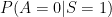
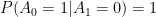
As we have binary variables, we have four different action-state combinations, $P(A=1|S=1)$ , $P(A=0|S=1)$ , $P(A=1|S=0)$ and $P(A=0|S=0)$ . As for $P(A)$ , our probability function is a discrete function over two discrete values of A 0 and 1. Now the “given” sign – “|” – means that our probability function (potentially) changes based on the values of the variables to right of the sign. Hence, we have one set of bars representing the probability distribution over the two values of A when S=0 and another set of bars representing the probability distribution over the two values of A when S=1.

In certain cases, we might define $P(A|S)$ as a function of S. Our output space is fixed – we can imagine probability on a y-axis and action as 0 or 1 on an x-axis. The shape of the function within this space depends on S.

Now, regardless of appropriateness, we can only start to have intelligence when $P(A|S) \neq P(A)$ , i.e. when the probability of taking an action given the state differs from just our probability of taking an action.

Through Bayes Theorum, we can rewrite $P(A|S)$ :

$P(A|S) = \frac{P(S|A)P(A)}{P(S)}$

For our inequality to hold, we see that $\frac{P(S|A)}{P(S)} \neq 1$ . In English, this means that the probability of the state of world given our action – $P(S|A)$ – needs to be different from the probability of the state of world without our action – $P(S)$ .

This makes nice poetic sense – if our actions didn’t make a difference we couldn’t be here.

Sense More

Some interesting things happen when we consider expanding our sensory repertoire.

Let’s consider that Dave has some mutated offspring. Let’s call that offspring “Susan”. Imagine that the offspring arises after a cosmic ray hits Dave’s DNA. The mutation causes Susan to be born with an additional sensory organ. Susan can sense the original state of the world, like Dave. For ease, let’s call this $S_{0}$ . But Susan can also sense an exciting new state, which we’ll call $S_{1}$ . Like, the original state, the new state can only be sensed in binary, so $S_{i} \in \{0, 1\}$ .

Are We Any Cleverer?

Now we can sense two states, does that make us any cleverer?

As before, we only make gains if the probability of acting differs given the two states, as compared to the one state: $P(A|S_{0}, S_{1}) \neq P(A|S_{0})$ . We also likely want our “two state” acting to differ from random action, such that $P(A|S_{0}, S_{1}) \neq P(A)$ .

Applying Bayes Theorem again, we get:

$P(A|S_{0}, S_{1}) = \frac{P( S_{0}, S_{1}|A)P(A)}{P(S_{0}, S_{1})}$

For the last inequality to hold, we need $\frac{P( S_{0}, S_{1}|A)}{P(S_{0}, S_{1})} \neq 1$ . For the first inequality, we need to break down this expression.

Independence

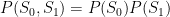
If our measured states are independent, we can start applying some mathematical tricks.

For example, if $S_{0}$ and $S_{1}$ are independent, then the joint probability of the two states equals the two separate probabilities multiplied together, or:

$P(S_{0}, S_{1}) = P(S_{0})P(S_{1})$

Conditional Independence

If our measured states are also conditionally independent, we can apply another trick.

Conditional independence means that two events are independent given, or conditional on, another third event. If the two measured states are independent given the action, we can say:

$P(S_{0}, S_{1}|A) = P(S_{0}|A)P(S_{1}|A)$

and

$P(S_{1}|A, S_{0}) = P(S_{1}|A)$

The latter expression is interesting. It says, if conditional independence holds, that the probability of our new state given an action and an old state is equal to just the probability of our new state given the action. We can think of this as saying that our action becomes the memory sink for our states or that the previous state only affects our current state through the medium of the action.

Simplifying

If we are able to say that the two measured states are both independent and conditionally independent given the action, then we can rewrite $P(A|S_{0}, S_{1})$ :

$P(A|S_{0}, S_{1}) = \frac{P(S_{0}|A)P(S_{1}|A)P(A)}{P(S_{0})P(S_{1})} = P(A|S_{0}) * \frac{P(S_{1}|A)}{P(S_{1})}$

In this case, for $P(A|S_{0}, S_{1}) \neq P(A|S_{0})$ to hold, we thus need $\frac{P(S_{1}|A)}{P(S_{1})} \neq 1$ . This is the same rule we found applies for $P(S|A)$ when we considered just one state.

In this case, we also see that we can reuse our old determination for $P(A|S_{0})$ (i.e. $P(A|S)$ as described above). We just condition our old finding based on our new information.

Feedback

It is also interesting to look at the expressions $\frac{P(S_{0}|A)}{P(S_{0})}$ and $\frac{P(S_{1}|A)}{P(S_{1})}$ . What do they relate to?

Well $P(S_{i}|A)$ is a form of feedback from the action to the state. This contrasts with our previously imagined scenario where we looked at the action given the state. $\frac{P(S_{i}|A)}{P(S_{i})}$ is a ratio expressing how the action changed the probability of the state. So Susan changes how she acts based on how her actions change her newly measured state.

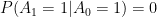
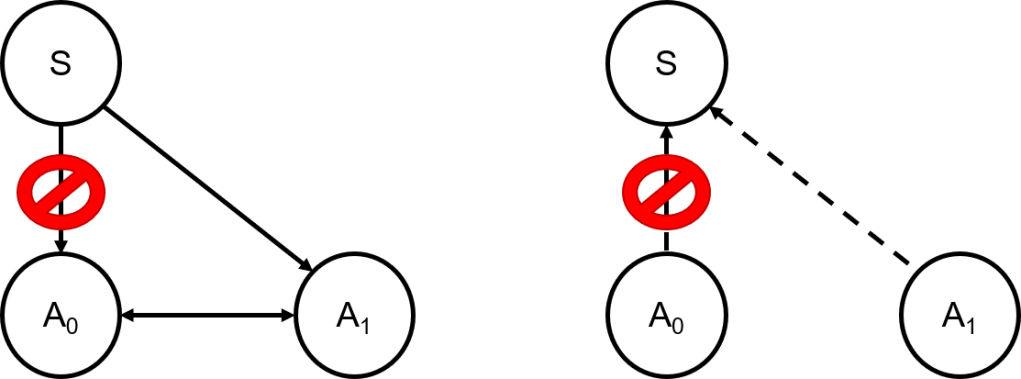
Bayesian Networks

In our simple toy configuration, the action A is both a “collider” and a “fork” depending on the direction we are considering. The “fork” pattern provides for conditional independence on the “fork”; in our case, looking from A backwards, A is the “fork” and $S_{0}$ and $S_{1}$ are conditionally independent given A.

Looking forwards, from the state to the action, as long as $S_{0}$ and $S_{1}$ have no causal connection, they are also independent. Looking backwards, from the action to the state, they are not independent unless we condition on A.

Separating Our States

If we know that $S_{0}$ and $S_{1}$ need to be independent, and that $S_{0}$ arises first, is there anything we can do to ensure this?

We can make a start by trying to make our states linearly independent. We can do this by transforming them such that they are uncorrelated. Two random variables are uncorrelated if their covariance is zero. We can make our states linearly independent by applying principal component analysis. We can consider a two state vector $\vec{S} =\begin{bmatrix} S_{0} \\ S_{1} \\ \end{bmatrix}$ and measure this over time:

$\mathbf{S} =\begin{bmatrix} S_{0}^{0} & S_{0}^{1} & S_{0}^{2} & \dots & S_{0}^{t} \\ S_{1}^{0} & S_{1}^{1} & S_{1}^{2} & \dots & S_{1}^{t} \\ \end{bmatrix}$

We can then use this to compute a covariance matrix, and then apply principal component analysis to develop a transformation matrix $U$ that may be applied to our original state vector $\vec{S}$ to obtain a decorrelated projection. The columns in U reflect the eigenvectors of the covariance matrix and the transformation seeks to make non-diagonal entries in the covariance matrix equal to 0 (i.e. decorrelating).

There is a great post from Stanford’s Computer Science department explaining this here.

Note: that PCA and the aforementioned post assume data with zero mean – our binary data has a non-zero mean so we require an additional mean-removal pre-processing step. It also makes sense to “whiten” any transformed data. This divides by the square roots of the eigenvalues such that the changes have unit (e.g. 1) variance.

More Action

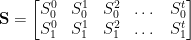
Let’s consider another mutation scenario. Imagine the cosmic ray hits Dave and the mutated sprog of Susan has two muscles rather than one. She can thus make two movements. Let’s call these $A_0$ and $A_1$ , where $A_0 = A$ (i.e. the first action is our old original action). Let’s also stick to the binary case, so $A_{i} \in \{0, 1\}$ .

Let’s also assume that Susan can control her new multi-muscles independently. This isn’t too unrealistic at this simple stage.

In a first scenario considering just a single state $S$ , Susan can just perform each action independently based on the state.

$P(A_0|S) = \frac{P(S|A_0)P(A_0)}{P(S)}$

$P(A_1|S) = \frac{P(S|A_1)P(A_1)}{P(S)}$

In a second scenario, we can imagine a constraint – only one of $A_0$ or $A_1$ may be active at one time. We can set this constraint by considering $P(A_0|A_1)$ and $P(A_1|A_0)$ . In these functions, to create an OR scenario, we want a probability function where $P(A_0=1|A_1=1)=0$ and $P(A_0=1|A_1=0)=1$ (and similarly $P(A_1=1|A_0=1)=0$ and $P(A_1=1|A_0=0)=1$ ).

IF (and it’s actually an unlikely IF), our state S and our action $A_0$ were independent and conditionally independent on $A_1$ , we could use a similar trick for the states above:

$P(A_1|S, A_0) = \frac{P(S, A_{0}| A_{1})P(A_{1})}{P(S, A_{0})}$

IF independent – $P(S, A_{0}) =P(S)P(A_0)$ and IF conditionally independent $P(S, A_{0}| A_{1}) = P(S|A_1)P(A_0|A_1)$ , so:

$P(A_1|S, A_0) = \frac{P(S, A_{0}| A_{1})P(A_{1})}{P(S, A_{0})} = \frac{P(S|A_1)P(A_{0}| A_{1})P(A_{1})}{P(S)P(A_{0})} = \frac{P(S|A_1)}{P(S)}*\frac{P(A_{0}| A_{1})P(A_{1})}{P(A_0)}$

$= \frac{P(S|A_1)}{P(S)}*P(A_1|A_0)$

The problem is we have neither independence nor conditional independence on $A_1$ . The state S and the first action $A_0$ are not independent as the probability of the first action depends on the state. The state S and the second action $A_1$ are also not conditionally independent given the first action $A_0$ , there is still a separate link between the state and the first action. This can be seen in the diagram below, where the left hand side represents “before an action” and the right hand side represents “after an action”.

It’s a shame because the simplified expression could have given us an expression to update our models for one state and one action, when an additional action is added.

If the conditions did hold, the probability of selecting an action from the new group would be dependent on how the actions interact – set by $P(A_1 | A_0)$ – and a non-unity factor for the new action – set by $\frac{P(S|A_1)}{P(S)}$ .

A similar expression could be drawn up for the first action $A_0$ .

If we were looking at how the probability of the old action changes, we would see that the new probability would be set by the existing non-unity factor for the old action – $\frac{P(S|A_0)}{P(S)}$ , i.e. how the state changes based on the action, and how the old action influences the new action $P(A_0 | A_1)$ .

Cutting the Cord

When considering the probability of the new second action in the context of the original first action $P(A_1|S, A_0)$ , we need to cut the causal chain from the state to the first action:

When considering the probability of the original first action in the context of the new second first action $P(A_0|S, A_1)$ , we need to cut the causal chain from the state to the second action:

Can we do this?!

Now things get interesting.

You probably know that correlation $\neq$ causation. This is because it is possible to have two random variables that have a correlation of 0 but that are still highly dependent. Why is this? It is because correlation only considers linear relationships between the variables. It is thus possible to have highly casual non-linear relationships that result in a correlation of 0. (This reminder sheet has a good example featuring a non-linear two-dimension function with a V-shape.)

But.

There are two things to consider.

First, if two random variables are jointly normally distributed a correlation of 0 does imply independence. This is interesting because the central limit theorem indicates that as we increase the number of samples, we may get something resembling a normal distribution.

Second, we can represent a function with a Taylor polynomial. This requires a sufficiently “well-behaved” function, which means that the function needs to be sufficiently continuously differentiable (at least up to the polynomial degree being applied). It indicates that complex functions can be imperfectly approximated using different levels of complexity. We can start we a linear approximation and progressively add higher order terms to get closer to the real function. This is shown for $\sin(x)$ below from the above link.

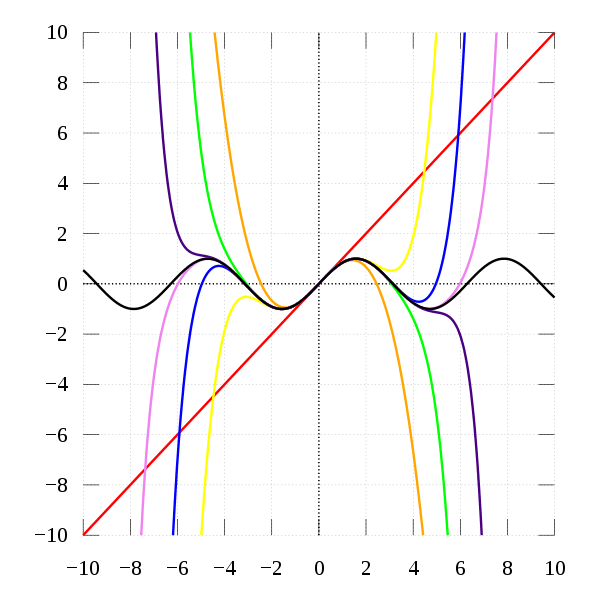
It may be that we can provide approximations to independence at different levels of complexity. The details of this can be looked at in a later post.

Looking Both Ways

So in this post, we looked at some simple state-action mappings.

We found that when we add additional states to control our actions, we could chain probabilities and develop rules for testing whether our additional information actually makes a difference to our actions.

It turns out that it doesn’t matter whether we look at things from the perspective of states or actions, similar probability rules apply. In both cases, when we extend the space of states or actions, we can use simple update rules if we can somehow ensure independence among the variables that form our context.

When considering an action in the context of multiple states, $P(A|S_0, S_1)$ , we needed independence between the two states and conditional independence on the variable in question (the action).

When considering an action that may be influenced by other actions and a state, $P(A_1|S, A_0)$ , we needed independence between the state and the other action, and conditional independence on the variable in question (the new action).

We also realised that we probably don’t have independence out-of-the-box. But there are hints that we can apply mathematical operations that result in an approximation of independence. In future posts we’ll consider whether these approximations are suitable for navigation within the real-world.