Folding Autoencoders

It’s nice when different ways of seeing things come together. This often occurs when comparing models of computation in the brain and machine learning architectures.

Many of you will be familiar with the standard autoencoder architecture. This takes an input , which may be an image (in a 2D or flattened 1D form) or another input array. It applies one or more neural network layers that progressively reduce the dimensionality of the output. These one or more neural network layers are sometimes called an “encoder”. This forms a “bottleneck” to “compress” the input (in a lossy manner) to form a latent representation. This latent representation is sometimes referred to as a hidden layer. It may be seen as an encoded or compressed form of the input.

A standard autoencoder may have a 1D latent representation with a dimensionality that is much less than the input dimensionality. A variational autoencoder may seek to learn values for a set of parameters that represent a latent distribution, such as a probability distribution for the input.

The autoencoder also has another set of one or more neural network layers that receive the latent representation as an input. These one or more neural network layers are sometimes called a “decoder”. The layers generate an output , which is a reconstruction of the input .

The whole shebang is illustrated in the figure below.

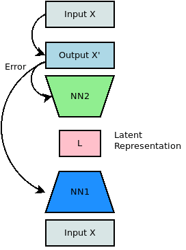
The parameters of the neural network layers, the “encoder” and the “decoder”, are learnt during training. For a set of inputs, the output of the autoencoder is compared with the input , and an error is back-propagated through the neural network layers. Using gradient descent to minimise the errors, an optimal set of parameters may be learnt.

As autoencoders do not require a labelled “ground-truth” output to compare with the autoencoder output during training, they provide a form of unsupervised learning. Most are static, i.e. they operate on a fixed instance of the input to generate a fixed instance of the output, and there are no temporal dynamics.

Now, I’m quite partial to unsupervised learning methods. They are hard, but they also are much better at reflecting “natural” intelligence; most animals (outside of school) do not learn based on pairs of inputs and desired outputs. Models of the visual processing pathway in primates, which have been developed over the last 50 years or so, all indicate that some form of unsupervised learning is used.

In the brain, there are several pathways through the cortex that appear similar to the “encoder” neural network layers. With a liberal interpretation, we can see the latent representation of the autoencoder as an association representation formed in the “higher” levels of the cortex. (In reality, latent representations in the brain are not found at a “single” flat level but are distributed over different levels of abstraction.)

If the brain implements some form of unsupervised learning, and seems to “encode” incoming sensory information, this leads to the question: where is the “decoder”?

This is where predictive coding models can help. In predictive coding models, predictions are fed back through the cortex to attempt to reconstruct input sensory information. This seems similar to the “decoder” layers of the autoencoder. However, in this case, the “encoder” and the “decoder” appear related. In fact, one way we can model this is to see the “encoder” and the “decoder” as parts of a common reversible architecture. This looks at things in a similar way to recent work on reversible neural networks, such as the “Glow” model proposed by OpenAI. The “encoder” represents a forward pass through a set of neural network layers, while the “decoder” represents a backward pass through the same set of layers. The “decoder” function thus represents the inverse or “reverse” of the “encoder” function.

This can be illustrated as follows:

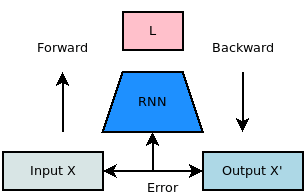
In this variation of the autoencoder, we effectively fold the model in half, and stick together the “encoder” and “decoder” neural network layers to form a single “reversible neural network”.

In fact, the brain is even cooler than this. If we extend across modalities to consider sensory input and motor output, the brain appears to replicate the folded autoencoder shown above, resulting in something that resembles again our original standard autoencoder:

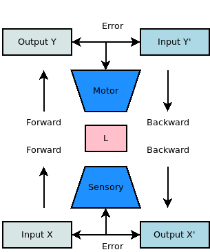
Here, we have a lower input “encoder” that represents the encoding of sensory input into a latent “associative” representation. A forward pass provides the encoding, while a backward pass seeks to predict the sensory input by generating a reconstruction . An error between the sensory input and the reconstruction is used to “train” the “encoder”.

We also have an upper output “decoder” that begins with the latent “associative” representation and generates a motor output . A forward pass decodes the latent “associative” representation to generate muscle commands.

The “backward” pass of the upper layer is more uncertain. I need to research the muscle movement side – there is quite a lot based on the pathology of Parkinson’s disease and the action of the basal ganglia. (See the link for some great video lectures from Khan Academy.)

In one model, somasensory input may be received as input , which represents the muscle movements as actuated based on the muscle commands. The backward pass thus seeks to reconstruct the latent “associative” representation from the input . The “error” may be computed at one or more of the input level (e.g. looking at the difference between and ) and the latent “associative” representation level (e.g. between the “sensory” input encoding and the “motor” input encoding). In any case there seem to be enough error signals to drive optimisation and learning.

Of course, this model leaves out one vital component: time. Our sensory input and muscle output is constantly changing. This means that the model should be indexing all the variables by time (e.g. , , , , and the latent “associative” representations). Also the forward and backward passes will occur at different times (the forward pass being available earlier than the backward pass). This means that our errors are also errors in time, e.g. between and for a common discrete time basis.

Many of the machine learning papers I read nowadays feature a bewildering array of architectures and names (ResNet, UNet, Glow, BERT, Transformer XL etc. etc.). However, most appear to be using similar underlying principles of architecture design. The way I deal with the confusion and noise is to try to look for these underlying principles and to link these to neurological and cognitive principles (if only to reduce the number of things I need to remember and make things simple enough for my addled brain!). Autoencoder origami is one way of making sense of things.