Here is a little notebook where I play around with converting images from a polar representation to a Cartesian representation. This is similar to the way our bodies map information from the retina onto the early visual areas.
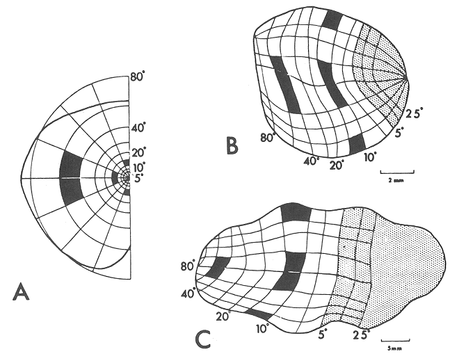
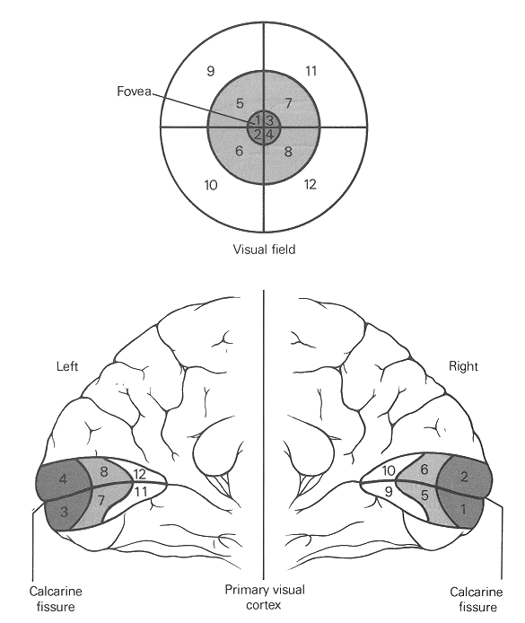
These ideas are based on information we have about how the visual field is mapped to the cortex. As can be seen in the above figures, we view the world in a polar sense and this is mapped to a two-dimensional grid of values in the lower cortex.
You can play around with mappings between polar and Cartesian space at this website.
To develop some methods in Python I’ve leaned heavily on this great blogpost by Amnon Owed. This gives us some methods in Processing I have adapted for my purposes.
Amnon suggests using a look-up table to speed up the mapping. In this way we build a look-up table that maps co-ordinates in polar space to an equivalent co-ordinate in Cartesian space. We then use this look-up table to look-up the mapping and use the mapping to transform the image data.
import math
import numpy as np
import matplotlib.pyplot as plt
def calculateLUT(radius):
"""Precalculate a lookup table with the image maths."""
LUT = np.zeros((radius, 360, 2), dtype=np.int16)
# Iterate around angles of field of view
for angle in range(0, 360):
# Iterate over diameter
for r in range(0, radius):
theta = math.radians(angle)
# Take angles from the vertical
col = math.floor(r*math.sin(theta))
row = math.floor(r*math.cos(theta))
# rows and cols will be +ve and -ve representing
# at offset from an origin
LUT[r, angle] = [row, col]
return LUT
def convert_image(img, LUT):
"""
Convert image from cartesian to polar co-ordinates.
img is a numpy 2D array having shape (height, width)
LUT is a numpy array having shape (diameter, 180, 2)
storing [x, y] co-ords corresponding to [r, angle]
"""
# Use centre of image as origin
centre_row = img.shape[0] // 2
centre_col = img.shape[1] // 2
# Determine the largest radius
if centre_row > centre_col:
radius = centre_col
else:
radius = centre_row
output_image = np.zeros(shape=(radius, 360))
# Iterate around angles of field of view
for angle in range(0, 360):
# Iterate over radius
for r in range(0, radius):
# Get mapped x, y
(row, col) = tuple(LUT[r, angle])
# Translate origin to centre
m_row = centre_row - row
m_col = col+centre_col
output_image[r, angle] = img[m_row, m_col]
return output_image
def calculatebackLUT(max_radius):
"""Precalculate a lookup table for mapping from x,y to polar."""
LUT = np.zeros((max_radius*2, max_radius*2, 2), dtype=np.int16)
# Iterate around x and y
for row in range(0, max_radius*2):
for col in range(0, max_radius*2):
# Translate to centre
m_row = max_radius - row
m_col = col - max_radius
# Calculate angle w.r.t. y axis
angle = math.atan2(m_col, m_row)
# Convert to degrees
degrees = math.degrees(angle)
# Calculate radius
radius = math.sqrt(m_row*m_row+m_col*m_col)
# print(angle, radius)
LUT[row, col] = [int(radius), int(degrees)]
return LUT
def build_mask(img, backLUT, ticks=20):
"""Build a mask showing polar co-ord system."""
overlay = np.zeros(shape=img.shape, dtype=np.bool)
# We need to set origin backLUT has origin at radius, radius
row_adjust = backLUT.shape[0]//2 - img.shape[0]//2
col_adjust = backLUT.shape[1]//2 - img.shape[1]//2
for row in range(0, img.shape[0]):
for col in range(0, img.shape[1]):
m_row = row + row_adjust
m_col = col + col_adjust
(r, theta) = backLUT[m_row, m_col]
if (r % ticks) == 0 or (theta % ticks) == 0:
overlay[row, col] = 1
masked = np.ma.masked_where(overlay == 0, overlay)
return masked
First build the backwards and forwards look-up tables. We’ll set a max radius of 300 pixels, allowing us to map images of 600 by 600.
backLUT = calculatebackLUT(300)
forwardLUT = calculateLUT(300)
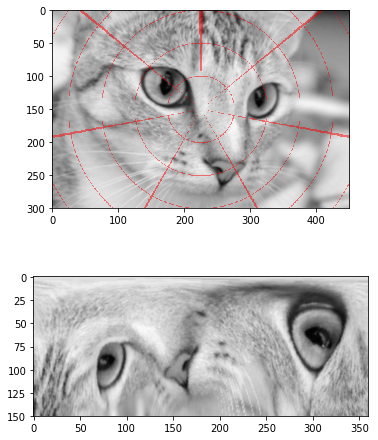
Now we’ll try this out with some test images from skimage. We’ll normalise these to a range of 0 to 255.
from skimage.data import chelsea, astronaut, coffee
img = chelsea()[...,0] / 255.
masked = build_mask(img, backLUT, ticks=50)
out_image = convert_image(img, forwardLUT)
fig, ax = plt.subplots(2, 1, figsize=(6,8))
ax.ravel()
ax[0].imshow(img, cmap=plt.cm.gray, interpolation='bicubic')
ax[0].imshow(masked, cmap=plt.cm.hsv, alpha=0.5)
ax[1].imshow(out_image, cmap=plt.cm.gray, interpolation='bicubic')
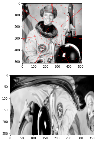
img = astronaut()[...,0] / 255.
masked = build_mask(img, backLUT, ticks=50)
out_image = convert_image(img, forwardLUT)
fig, ax = plt.subplots(2, 1, figsize=(6,8))
ax.ravel()
ax[0].imshow(img, cmap=plt.cm.gray, interpolation='bicubic')
ax[0].imshow(masked, cmap=plt.cm.hsv, alpha=0.5)
ax[1].imshow(out_image, cmap=plt.cm.gray, interpolation='bicubic')
img = coffee()[...,0] / 255.
masked = build_mask(img, backLUT, ticks=50)
out_image = convert_image(img, forwardLUT)
fig, ax = plt.subplots(2, 1, figsize=(6,8))
ax.ravel()
ax[0].imshow(img, cmap=plt.cm.gray, interpolation='bicubic')
ax[0].imshow(masked, cmap=plt.cm.hsv, alpha=0.5)
ax[1].imshow(out_image, cmap=plt.cm.gray, interpolation='bicubic')
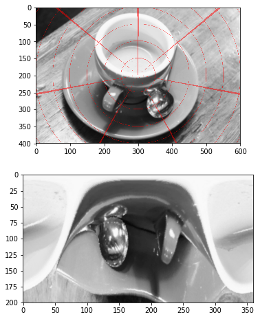
In the methods, the positive y axis is the reference for the angle, which is extends clockwise.
Now, within the brain the visual field is actually divided in two. As such, each hemisphere gets half of the bottom image (0-180 to the right hemisphere and 180-360 to the left hemisphere).
Also within the brain, the map on the cortex is rotated clockwise by 90 degrees, such that angle from the horizontal eye line is on the x-axis. The brain receives information from the fovea at a high resolution and information from the periphery at a lower resolution.
The short Jupyter Notebook can be found here.
Extra: proof this occurs in the human brain!

