Predicting the Future

The rise of machine learning and developments in neuroscience hint that prediction is key to how brains navigate the world. But how could this work in practice?

Let’s ignore neuroscience a minute and just think how we would manually predict the future. Off the top of my head there appear to be three approaches, which we will look at below.

Instantaneous Prediction Using Rates of Change

In the physical world, one way to predict the future is to remember our secondary school physics (or university kinematics). For example, if we wanted to predict a position of an object moving along one dimension, we would attempt to find out its position, speed and acceleration, and use equations of motion. In one-dimension, speed is just a measure of a change of position over time (a first-order differential with respect to time). Acceleration is a measure of change of speed over time (a second order differential with respect to time, or a change in a change).

In fact, it turns out the familiar equations of motion are actually just a specific instance of a more general mathematical pattern. James Gregory, Brook Taylor and Colin Maclaurin formalised this approach in the 17th and 18th centuries, but thinking on this issue goes back at least to Zeno, Democritus and Aristotle in ancient Greece, as well as Chinese, Indian and Middle Eastern mathematicians. In modern times, we generally refer to the pattern as a Taylor Series: a function may be represented as an infinite sum of differentials about a point.

For example, our normal equation for distance travelled in one dimension is 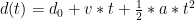, where d is distance, v is velocity and a is acceleration. In this case, velocity is our first differential – a first-order rate of change of distance with time – and acceleration is our second differential – a second-order rate of change of distance with time (or a rate of change of velocity). We know from school that if we have constant velocity, a is zero and we just have . What isn’t stressed as much is that the equations learnt by every school kid are for a single dimension with at worst constant acceleration. It is not until university that the veil begins to be removed and we realise that if we have changing acceleration (third-order changes), we need to add another term, and that we can continue this ad-nausem.

As you move into more advanced engineering and physics classes, you are also taught how to extend the equations of motion into two or three dimensions. When we have movement in three-dimensional space, we can model points in spacetime using four-dimensional vectors (). As we move into the multidimensional case, we can look at how each dimension changes with respect to each other dimension for the point. For example, changes in an x-dimension with time (t) may resemble our one-dimensional speed. However, in the multivariate case we now can determine changes in the y and z direction with time. Hence, our velocity becomes a vector indicating how the x, y and z dimensions of the point change over time. Because the directions of modelled Cartesian space are orthogonal, we can analyse them separately.

We will stop here for now but we can also go further. If we can guess at the mass of an object, we can predict an acceleration using . Hence, our brains can begin to build a suite of approximated functions that predict the rates of change from additional data or latent variables discerned from the data.

Neural Units

So let’s return to thinking about brains. Populations of neurons in our brains do not have god-like powers to view an objective reference frame that depicts spacetime. Instead, they are fixed in space, and travel through time. What they can be is connected. But even this must be limited by practical reality, such as space and energy.

In fact, we can think about “neural units”, which may be a single neuron or a population of neurons. What makes a neural unit “a unit” is that it operates on a discrete set of information. In an image processing case this may be a pixel, in a audio processing example this may be a sample in time, or a frequency measurement.

Now the operation of a neural unit begins to resemble the assumptions for the Taylor Series: it is the point around which our function is evaluated, and all we need is local information relating to our derivatives. We’ll ignore for now the fact that our functions may not be infinitely differentiable about our unit, as it turns out approximations often seem to work fine.

So bringing this all together, we see that a neural unit may be able to (approximately) predict future activity, either of itself in time, or its neighbours in space, by determining local rates of change of different orders.

For example, if we consider the image intensity of a single pixel, we can see that a neural unit may be able to predict the intensity of that pixel at a future time, if there are patterns in the rates of change. For example, if the pixel intensity is increasing at a constant rate, r, then the intensity at a future time, t, may be determined like our velocity above: .

Linear Approximations

Another way of viewing the same thing is to think about linear approximations.

What are linear approximations? They are just functions where the terms are linear, i.e. are not a power. In a Taylor Series this means chopping off everything past a first order differential. Now, if a car is accelerating towards you, assuming a constant velocity is going to be a very costly mistake. But what is surprising is that a fair bit of engineering is built upon linear approximations. In fact, even now some engineers pull a funny face and start sweating when you move away from linear models. It turns out that a significant portion of the world we live in has first order patterns.

If you go up a little way to include second order patterns, you find that another large chunk of the world can be approximated there. This is most visible in the equations of motion. Why can we stop with second order acceleration terms? Because gravity is constant at 9.8m/s. Until recently, the main things that displayed changing accelerations were animals.

So can we just throw away higher order terms? Not exactly. One issue with a power series is that as we try to predict further from our point or neural unit, higher order differentials become more important. For example, looking forward beyond the first few immediate units and the higher terms will dominate the prediction. Often this is compounded by sensory inaccuracy, the rates of change will never be exact, and errors in measurement are multiplied by the large high-order terms.

So what have we learnt? If we are predicting locally, either in space or in time, in a world with patterns in space-time, we can make good approximations using a Taylor series. However, these predictions become less useful in a rapidly changing world where we need to predict over longer distances in space and time.

Prediction Using Cycles

Many of the patterns in the natural world are cyclical. These include the patterns of day and night caused by the rotation of the Earth upon its (roughly) north-south axis, the lunar months and tides caused by the rotation of the moon around the Earth, and the seasons caused by the rotation of the Earth around the sun. These are “deep” patterns – they have existed for the whole of our evolutionary history, and so our modelled at least chemically at a low-level in our DNA.

There are then patterns that our based on these patterns. Patterns of sleep and rest, of meal times, of food harvest, of migration, or our need for shelter. Interestingly many of these patterns are interoceptive patterns, e.g. relating to an inner state of our bodies representing how we feel.

The physical world also has patterns. Oscillations in time generate sound. Biological repetition and feedback cycles generates cyclical patterns, such as the vertical lines of light-and-dark observed looking into a forest or the stripes on a zebra.

How do we make predictions using cycles?

Often we have reference patterns that we apply at different rates. In engineering, this forms the basis of Fourier analysis. The rate of repetition we refer to as “frequency”. We can then build up complex functions and signals by the addition of simple periodic or repeating functions with different magnitudes and phases. In mathematics the simple periodic functions are typically the sine or cosine functions.

So if we can use a base set of reference patterns, how does working in the frequency domain help prediction?

In one dimension the answer is that we can make predictions of values before or after a particular point based on our knowledge of the reference functions, and estimates for magnitudes and phases. For a signal that extends in space or time, we only need to know a general reference pattern for a short patch of space or time, stretch or shift it and repeat it, rather than trying to predict each point separately and individually.

When our brain attempts to predict sounds, it can thus attempt to predict frequencies and phases as opposed to complex sound waveforms. In space, things are less intuitive but apply similarly. For example, repeating patterns of intensity in space, such as stretches of light and dark lines (the stripes on a zebra) may be approximated using a reference pattern of one light and one dark line, and then repeating the pattern at an estimate scale, strength and phase. Many textures can be efficiently represented in this way (think of the patterns on plants and animals).

Thinking about neural units, we can see how hierarchies of units may be useful to implement predictions of periodic sequences. We need a unit or population of units to replicate the reference pattern, and to somehow represent an amplitude and phase.

Statistical Prediction

A third way to make predictions is using statistics and probability.

Statistics is all about large numbers of measurements (“big data”, when that was trendy). If we have large numbers of measurement we can look for patterns in those numbers.

Roll a six-sided dice a few times and you will record what look like random outcomes. We might have three “4s”, and two “1s”. Roll a dice a few million times and you will see that each of the six numbers occur in more-or-less similar proportions: each number occurs 1/6th of the time. The probability of rolling each number may then be represented as “1/6”.

Rates of change are fairly useless here. This is because we are dealing with discrete outcomes that are often independent. These “discrete outcomes” are also typically complex high-order events (try explaining “roll a dice” to an alien). If you were to measure the change in rolled number (e.g. “4” on roll 1 minus “1” on roll 0 = 3), this wouldn’t be very useful. Similarly, there are no repeating patterns in time or space that make Fourier analysis immediately useful for prediction.

Thinking about a neural unit, we can see that probability may be another way to predict the future. If a neural unit received an intensity for a pixel associated with the centre of a dice, it could learn that the intensity could be 0 or 1 with a roughly 50% likelihood (e.g. numbers 1, 3 and 5 having a central dot, which is absent from numbers 2, 4 and 6). If it got an intensity of 0.5, something strange has happened.

Probability, at its heart, is simply a normalised weight for a likelihood of an outcome. We use a value between 0 and 1 (or 0 and 100%) so that we can compare different events, such as rolling a dice or determining if a cow is going to charge us. In a discrete case, we have a set of defined outcomes. In a continuous case, we have a defined range of outcome values.

How Do Rates of Change and Probabilities Fit Together?

Imagine a set of neural units relate to a pixel in an image. For example, we might look at a nearest pixel to a centre of a webcam image.

In this case, each neural unit may have one associated variable: an intensity or amplitude. Say we have an 8-bit image processing system, so the neural unit can receive a value between 0 and 255 representing a measured image characteristic. This could be a channel measurement, e.g. an intensity for lightness (say 0 is black and 255 is white) or for “Red” (say 0 is not red and 255 is the most red) or an opponent colour space (say 0 is green and 255 is red).

Now nature is lazy. And thinking is hard work. Our neural units want to minimise any effort or activity.

One way to minimise effort is to make local predictions of sensory inputs, and to only pass on a signal when those predictions fail, i.e. to output a prediction error.

A neural unit could predict its own intensity at a future time or the intensity of one of its neighbours, e.g. in space. If a neural unit receives an intensity in , it can compute an overall intensity prediction based on time and space prediction and then determine an error between them .

One way to approximate a rate of change is to simply compare neighbouring units in space, or current and past values in time. To compute higher orders, we just repeat this comparison on previously computed rates of change.

If they are arranged in multiple layers, our neural units could begin to predict cyclical patterns. Over time repeated patterns of activity could be represented by the activity of a single set of neural units and a reference to the underlying units that show this activity, e.g. as scaled or shifted. This would be lazier – we could just copy or communicate the activity of the single unit to the lower neural units.

Probability may come into play when looking at a default level of activity for a given context. For example, consider an “at rest” case. In many animals the top of the visual field is generally lighter than the bottom of the visual field. Why is this? Because the sky is above and the ground is below. Of course, this won’t always be the case, but it will be a general average over time. Hence, if you have no other information, a neural unit in the upper visual field would do wise to err on a base level of intensity that is higher (e.g. lighter) that a neural unit in the lower visual field. This also allows laziness in the brain. A non-light intensity signal received by the neural unit in the upper visual field is more informative than a light intensity signal as it is more unlikely. Hence, if there is a finite amount of energy, the neural unit in the upper visual field wants to use more energy to provide a signal in the case of a received non-light intensity signal than in the case of a received light intensity signal. Some of you would spot that we are now moving into the realms of (Shannon) entropy.

In the brain then, it is likely that all these approaches for prediction are applied simultaneously. Indeed, it is probable that the separate functions are condensed into common non-linear predictive functions. It is also likely that modern multi-layer neural networks are able to learn these functions from available data (or at least rough approximations based on the nature of the training data and the high-level error representation).