Invariance, Scale and Prediction

Consider the Cow

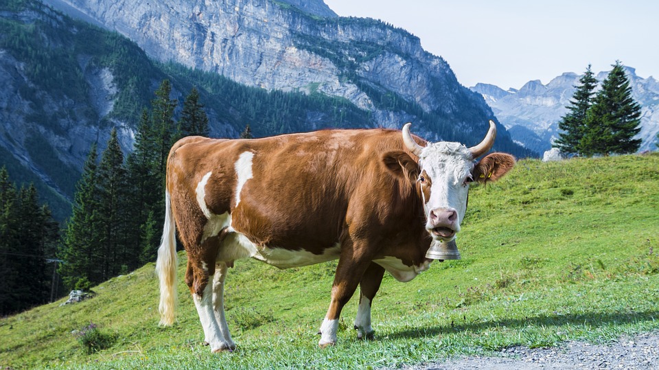
Consider a cow in the distance.

Now consider a cow up close.

Why do we see both these images as a “cow”, when the size of the image clearly differs?

If we imagine that information from our retina is passed to many different processing areas of the visual cortex, why do we still see a cow regardless of the number of processing units that receive “cow-related” image information?

Invariance

How different images can relate to common “objects” involves the study of invariance: how a varying input can lead to a constant output. There are multiple forms of invariance, including: scale invariance (the cows as above), angle invariance (why do we see a cow despite walking around the cow) and time invariance (an image of a cow in 5 seconds is still showing a cow).

Let’s think for a moment about scale invariance. How could this be implemented?

One clue comes as we consider an image at different resolutions:

If we scale up a distant object we see it is the same as downsampling a closer object.

Our limit is our resolution – the smallest representation of an object is one pixel, which doesn’t provide that much information. We can imagine a case where we double the width and height of an image area at a number of stages to provide a set of scales of different resolutions. For example, an object may be represented by:

• 1×1 area (1 pixel) at scale S0;
• 2×2 area (4 pixels) at scale S1;
• 4×4 area (16 pixels) at scale S2;
• 8×8 area (64 pixels) at scale S3;
• 16×16 area (256 pixels) at scale S4;
• 32×32 area (1024 pixels) at scale S5;
• 64×64 area (4096 pixels) at scale S6;
• 128×128 area (16384 pixels) at scale S7;
• 256×256 area (65536 pixels) at scale S8; and
• 512×512 area (262144 pixels) at scale S9.

Here we only need 10 levels to cover a wide array of different sizes. Indeed, we have a logarithmic scale with base 2, as we go from scale level 0 to scale level 9 we go from pixels to pixels.

How can we compare these different scales? How can we know that an object that is centred in an image at scale S9 is the same object as is centred in the image at scale S2?

The answer is that we can filter the higher resolution images. In particular, we can downsample the images at a higher scale such that they resemble images at a lower scale.

Filtering

How can we perform this filtering?

One way is to apply a Gaussian filter to provide a Gaussian blur. We can then take an average or max value for an image patch at a higher scale and compare it with a single pixel at a lower scale. This is actually the basis of the Scale-Invariant Feature Transform (SIFT), a feature extraction technique that was popular in the pre-deep learning days.

From an image processing viewpoint, we can generate each scale by convolving an original image with different Gaussian kernels, i.e. different matrix representations of a symmetric two-dimensional Gaussian curve.

The first few stages of SIFT algorithm are very similar to what we want to do here. In the SIFT algorithm, we take an image, replicate it n times (to generate an image set for an “octave“) and then apply a different scale Gaussian filter to each of the n images (getting progressively blurry). We then take the difference of adjacent images in n for each octave to generate a set of n-1 Gaussian differences for each octave. At this point in the SIFT algorithm they iterate through the pixels looking for local extrema. We will stop here for the moment.

In the SIFT algorithm, you can apply a Gaussian filter to a set of images in a first octave, and then subsample these images to create the images of different octaves. This is similar to navigating the scales above – but going down rather than up. The technique of generating multiple images is often called generating an image pyramid.

AI Shack has a nice walkthrough of SIFT: http://aishack.in/tutorials/sift-scale-invariant-feature-transform-scale-space/.

Image Pyramids

There are multiple ways to generate an image pyramid. Certain approaches may be seen as approximations of other approaches. 

• in a first approach, an original image may be subsampled;
• in a second approach, a mean pixel value for a given patch of pixels (e.g. a 2×2 or 3×3 grid) may be computed and used as a lower level pixel value; and
• in a third approach, a Gaussian mask may be applied before subsampling.

In true Blue Peter style, here are some examples I prepared earlier (with a cat rather than a cow I’m afraid):

Gaussian filters allow us to perform some nice computational tricks. To prevent aliasing, engineers recommend that we apply a Gaussian blur before subsampling. This lecture – http://www.cse.psu.edu/~rtc12/CSE486/lecture10.pdf – explains more.

For example:

Thinking of the Mathematics

Convolution can be implemented using a large matrix multiplication. The Stanford Computer Science Department has an excellent blogpost I keep returning to that describes this: http://cs231n.github.io/convolutional-networks/ .

For me, the most illuminating discovery was realising that the convolution operation may be represented by generating a matrix with multiple shifted versions of either the convolution filter or the signal and then multiplying that by the other of the signal or the convolution filter. This is nicely explained in the Wikipedia page on Toeplitz Matrices – https://en.wikipedia.org/wiki/Toeplitz_matrix#Discrete_convolution.

Remembering the size rules for matrix multiplication helps understand the operation here. If you have a first matrix M1 of size X1 by Y1 and a second matrix M2 of size X2 by Y2 (where we will refer to ROWS by COLUMNS to match numpy), when performing M1*M2 you need the inner dimensions to match and you get a result equal to the outer dimensions, so (X1 * Y1) * (X2 * Y2) – Y1 and X2 need to be the same size (or the width/number of columns of M1 needs to match the height/number of rows of M2) and you get a result of size X1 * Y2.

In the above examples, for a signal of length n and a filter of length m, you need to shift your filter n times (as represented by the columns of the upper figures) or shift your signal m times (as represented by the rows of the lower figure).

I find the second version that shifts the signal easier to conceptually understand. The number of rows of the second matrix (M2) equal the number of columns of the first matrix (i.e. m). And on every row we are shifting x by 1, meaning by the time we reach the last row we would have shifted m times (i.e. m leading 0s) before having the n values of x. Hence, the second matrix is of width m+n. (Similar logic applies to the first case, so the height/number of rows of the first matrix M1 in the first case is also m+n.)

These examples are all a 1D filter case with a stride of 1. If we are looking at Gaussian filtering, the convolution filter h is a 1D Gaussian kernel (its values plot out a “normal” or Gaussian distribution). I found understanding this simple case a great help for understanding the more complex 2D, multiple filter case used for standard convolutional neural network convolution.

Prediction

The general idea of the predictive brain is that we want to predict our sensory inputs. How does this relate to scale invariance?

If you have a high-level neural representation of an object, sometimes called a “code” in the parlance of autoencoder architectures, you want to be able to predict what that object will look like at different scales. For example, if when you are looking at the world and your brain computes “this is the kind of situation where I might find a cow“, the “cow” may appear as shapes of different sizes depending on its relative location. So we may have a top-down input that “primes” processing units at each of the scales.

Let’s ignore neuroscience a minute and just think how we would manually do this.

What are we trying to predict?

It’s a good question – at a high level we might be trying to predict what object it is (classification) or how to move our body to avoid or intercept. In fact our brains try to do both in parallel via the ventral (bottom of brain from the back of the head around to the ears) and dorsal (top of head from the back of the head over the top-ish to the eyebrows) processing pathways. In the latter case, we want to minimise the error in the movement to the object, or our prediction of where our body is and should be. This can be based on a difference between where we move our body to (as observed) and where we were trying to move our body to (the desired position). In the former case, we can acquire further information that tells us whether our classification is correct (e.g., from sounds, smells, tastes etc. – the latter being particularly important for foodstuff foraging).

An image is typically defined as a two-dimensional array, e.g. where x and y co-ordinates indicate a pixel value I(x, y). The pixel value is generally just an activation, it may represent a lightness value, an opponent colour value, or something vaguer, like a differential.

However, we don’t only see images. We see images, in time. Hence, we actually have a three-dimensional array, where x and y and t co-ordinates indicate a pixel value I(x, y, t). Prediction then may occur along these dimensions.

So, what is the laziest visual prediction of an object?

For example, consider the cow again. If I imagine a “cow”, we know that the lower visual circuits of the brain activate in a similar way to when we see a cow (it’s easier with your eyes shut as you have no conflicting input information). Now the laziest representation is that which displays the whole object within the visual field, at a size that biases our centre of vision (where the fovea is located). This also funnily enough seems to represent an “arms length” position of the object. Of course we can’t hold a cow at arms length, but we mean imagine the cow is of a size that is similar to a smaller object held at arms length. You can actually try this at home: get a variety of objects and you will be aware that there is a comfortable viewing distance, which is about arms length (see also how we view information on computer monitors, phones and in books).
If we bring the object closer than this laziest length, we start to break the object into component parts, despite some awareness that this relates to, or is in the context, of the arms length object.

So a smart and lazy way to predict, over both space and time, is to predict a lowest resolution first and fill in the detail in time. Indeed, in the visual circuitry, there is no high resolution representation in the periphery of our field of view, so all we have is a low resolution impression.

Another good approach is to look for a common pattern (e.g., the shape of a cow) at multiple scales in parallel. This is what SIFT does, it looks for a best match across different scale representations.