Swift Taylor Approximations

This post continues my explorations of simple intelligence.

In this post, we’ll consider some elementary sensing cells. We’ll then look at whether we can apply local function approximators.

Sensors

Consider a set of sensing cells, which we’ll call “sensors”.

We have N sensors, where each sensor measures a value over time. This value could be a magnitude or intensity, such as a lightness or colour intensity for vision, a frequency magnitude for sound, or a level of cell damage for pain. We’ll assume the N sensors form a small group – possibly a receptive field. The N sensors could therefore form part of a cortical column.

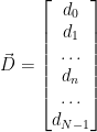
We can represent the set of N sensors as a column vector. The column vector represents a measurement at one point in time. We’ll represent each sensor using an index $n$ . You could call each sensor a “feature”. We’ll represent time using a set of discrete time steps, where a particular time step is represented by the variable $t$ . Hence, we have something like:

$\vec{S_t} = \begin{bmatrix} s^t_{0} \\ s^t_{1} \\ \dots \\ s^t_{n} \\ \dots \\ s^t_{N-1} \end{bmatrix}$

Note: we’ll start counting things in this post from 0 (as this matches Python implementations). This means that if we have N sensors our vector ends with the N-1th entry.

Measured Functions

To start, we can imagine that the measurements of each sensor conform to a function.

The function may be considered a function of time that is specific to the sensor. This gives us: $s^t_n = f_n(t)$

To makes things easier, we’ll consider a quantised or discrete time base. Hence, t has integer values from 0 to $\infty$ .

If we collect batches of samples (i.e. measurements) from the sensors over time, we can pop these into a matrix form $\mathbf{S}$ . If our set of sensor measurements at time $t$ is a column vector $\vec{S_t}$ , where each row relates to a different sensor, then we can stack these columns horizontally over a time period with P time steps to generate an N by P (rows by columns) matrix:

$\mathbf{S} = \begin{bmatrix} s^0_{0} & s^1_{0} & \dots & s^t_{0} & \dots & s^{P-1}_{0}\\ s^0_{1} & s^1_{1} & \dots & s^t_{1} & \dots & s^{P-1}_{1} \\ \dots & \dots & \dots & \dots & \dots & \dots \\ s^0_{n} & s^1_{n} & \dots & s^t_{n} & \dots & s^{P-1}_{n} \\ \dots & \dots & \dots & \dots & \dots & \dots \\ s^0_{N-1} & s^1_{N-1} & \dots & s^t_{N-1} & \dots & s^{P-1}_{N-1} \end{bmatrix}$

(Note: I use P instead of T to avoid confusion with the transpose operator – T – which we’ll use later.)

Covariance

We can use $\mathbf(S)$ to calculate a covariance matrix $\mathbf{M}$ for the time period.

Now officially we shouldn’t do this. Our samples are not I.I.D. – independent and identically distributed. Indeed, our function assumes there is some dependence over time. It is also likely that probability distributions for the sensor intensity change with time. But let’s play around for just one post to see what happens when we mix the streams. In effect, we are considering each time step to be an independent trial with a common intensity probability distribution, yet also considering each sensor to record a function over time.

Mean Adjustments

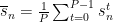
When dealing with a number of statistical samples, it is recommend to start by adjusting the data to have a mean of zero. This means that we need to subtract the mean measurement of each sensor over the time period from the sensor readings for that sensor. Let’s call the mean for the time period $\overline{S}$ – this is column vector of length N (i.e. size N by 1). The nth entry in $\overline{S}$ is calculated as:

$\overline{s}_n = \frac{1}{P}\sum_{t=0}^{P-1} s^t_n$

We need to be a little careful. Because we are using an discrete integer time base where a time index is incremented by 1 at each time step, we can substitute P for the number of samples. If we were using a different time base, this would not be possible.

To get a mean adjusted set of measurements, we perform a column-wise subtraction:

$\vec{S^{\prime}_t} = \vec{S_t} - \overline{S}$

This gives us an adjusted data sample matrix $\mathbf{S'}$ .

Covariance Calculation

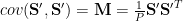
Given the adjusted data sample matrix $\mathbf{S'}$ , we can compute our covariance matrix as:

$cov(\mathbf{S'}, \mathbf{S'}) = \mathbf{M} = \frac{1}{P}\mathbf{S'}\mathbf{S'}^T$

(Note: sometimes this is written as simply $var(\mathbf{S'})$ but I’ll explicitly put in that we are looking at covariance between the sensors as later we may consider covariance between our sensors and something else. Or to put another way, here we are determining a cross-covariance matrix with ourselves or a variance matrix.)

In the above calculation, we have a first matrix $\mathbf{S'}$ of size N by P and a second matrix $\mathbf{S'}^T$ of size P by N (the transpose operation just swaps our rows and columns over). The result is a matrix $\mathbf{M}$ of size N by N, i.e. where an ijth value in the matrix represents the covariance of the ith sensor with the jth sensor or a measure of how the ith sensor changes with the jth sensor.

Now we’ll just park our covariance matrix for a moment. We’ll need it later when we look at decorrelating the sensor readings. But now we’ll go on a little detour into function approximators…

Taylor Polynomials

Let’s return to our sensor measurements over time.

From before, we considered that we can model each sensor with a function that changes over time: $s^t_n = f_n(t)$ .

Consider a moment. This one. That one. Any moment.

We can approximate the sensor function $s^t_n$ at that moment using a Taylor Series Expansion. If we call the moment $m$ we have:

$f_n(x) = f_n(m) + f'_n(m)(x-m)+\frac{f''_n(m)}{2!}(x-m)^2 + \frac{f'''_n(m)}{3!}(x-m)^3 + \dots + \frac{f^{k}_n(m)}{k!}(x-m)^k + \dots$

If we consider a moment at t=0 then this becomes a Maclaurin series:

$f_n(x) = f_n(0) + f'_n(0)(x)+\frac{f''_n(0)}{2!}(x)^2 + \frac{f'''_n(0)}{3!}(x)^3 + \dots + \frac{f^{k}_n(0)}{k!}(x)^k + \dots$

Now, we can use this to determine an approximation to the function at the moment. As the series is a sum of terms we can take different groups of successive terms as different levels of estimation. The first term is a relatively poor estimate, the first and second terms are better but still reasonably poor, the first to third terms are better again but still not as good as having more terms etc. You may have come across a similar approach when considering the mathematical notion of moments (although these are unrelated to our “moment” in time). The underlying idea crops up a fair amount across different fields, annoyingly referred to as different things in each field.

The moment in time matters because the accuracy of approximations is centred around the moment. The further away from the moment, the greater the divergence from the actual function. You can see this in the following example of approximating $\sin(x)$ around x=0 from Wikipedia:

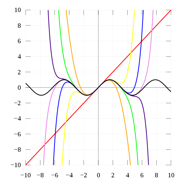
The approximation becomes increasingly bad the further we stray from 0.

Now if we consider the Maclaurin series of the function $f_n(x)$ and look at the function as a time-series function where $x = t$ then we can simplify a little with the following expression:

$s^t_n \approx a_n + b_n*t + c_n*t^2 + d_n*t^3 + \dots$

We can also consider the set of sensor signals as separate functions that are approximated with different coefficients:

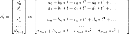
$\vec{S_t} = \begin{bmatrix} s^t_{0} \\ s^t_{1} \\ \dots \\ s^t_{n} \\ \dots \\ s^t_{N-1} \end{bmatrix} \approx \begin{bmatrix} a_0 + b_0*t + c_0*t^2 + d_0*t^3 + \dots \\ a_1 + b_1*t + c_1*t^2 + d_1*t^3 + \dots \\ \dots \\ a_n + b_n*t + c_n*t^2 + d_n*t^3 + \dots \\ \dots \\ a_{N-1} + b_{N-1}*t + c_{N-1}*t^2 + d_{N-1}*t^3 + \dots \end{bmatrix}$

We can then rewrite this in tensor form.

(Aside: these expressions may remind you of the equations of motion – indeed for motion these form of approximations work well with low powers such as 1 or 2. It’s interesting to consider that motion and orientation within space are some of the earliest tasks that require intelligence.)

Now time series data provides for some interesting tricks. A first is that all our sensors are operating according to a common time base. Hence, we have a set of vector * scalar multiplications:

$\vec{S_t} \approx \vec{A} + \vec{B}*t + \vec{C}*t^2 + \vec{D}*t^3 + \dots$

Where:

$\vec{A} = \begin{bmatrix} a_0 \\ a_1 \\ \dots \\ a_n \\ \dots \\ a_{N-1} \end{bmatrix}$ , $\vec{B} = \begin{bmatrix} b_0 \\ b_1 \\ \dots \\ b_n \\ \dots \\ b_{N-1} \end{bmatrix}$ , $\vec{C} = \begin{bmatrix} c_0 \\ c_1 \\ \dots \\ c_n \\ \dots \\ c_{N-1} \end{bmatrix}$ , $\vec{D} = \begin{bmatrix} d_0 \\ d_1 \\ \dots \\ d_n \\ \dots \\ d_{N-1} \end{bmatrix}$ etc.

Now we can consider the form of our mean adjusted vector $\vec{S^{\prime}_t}$ .

First, let’s determine our mean vector using the Taylor polynomial:

$\overline{S} = \frac{1}{P}\sum_{t=0}^{P-1} s^t_n = \frac{1}{P}\sum_{t=0}^{P-1} (\vec{A} + \vec{B}*t + \vec{C}*t^2 + \vec{D}*t^3 + \dots)$

$\overline{S} = \vec{A}*\frac{P}{P} + \vec{B}*\frac{1}{P}\sum_{t=0}^{P-1}t + \vec{C}*\frac{1}{P}\sum_{t=0}^{P-1}t^2+\vec{D}*\frac{1}{P}\sum_{t=0}^{P-1}t^3 + \dots$

$\overline{S} = \vec{A}+ \vec{B}*\overline{t} + \vec{C}*\overline{t^2}+\vec{D}*\overline{t^3}+ \dots$

This assumes we are evaluating the mean using the function approximation about 0.

What we are left with for the mean signal $\overline{S}$ is an expression similar to our original expansion for $t$ but this time being evaluated in terms of the means of each term (e.g. $\overline{t}, \overline{t^2}, \overline{t^3}$ etc.).

Now if we look at a mean adjusted signal using our new expression for the mean:

$\vec{S^{\prime}_t} = \vec{S_t} - \overline{S} \approx (\vec{A} + \vec{B}*t + \vec{C}*t^2 + \vec{D}*t^3 + \dots) - (\vec{A}+ \vec{B}*\overline{t} + \vec{C}*\overline{t^2}+\vec{D}*\overline{t^3}+ \dots)$

$\vec{S^{\prime}_t} \approx \vec{B}(t-\overline{t}) +\vec{C}(t^2-\overline{t^2}) +\vec{D}(t^3-\overline{t^3}) + \dots$

Now this reminds me a little of our original Taylor series expansion, only performed around the mean time period.

Rebasing

The expression above gives us a clue that we might reformulate our series sums around different moments within our time period.

If we have an incremental integer time base, from 0 to P-1, there are P integer values, where the mean value is:

$\overline{t} = \frac{1}{P}\sum_{t=0}^{P-1}t = \frac{(P-1)P}{2}$

(Note: We can use Faulhaber’s formula for the sum.)

But if we shift the P time points to be centred on t=0, we get $\overline{t} = 0$ .

To play nice with an integer time base, we’ll look at P points that include 0. For example, we can run from -(P-1)/2 to (P-1)/2 (the “-1” enters in because we have “0” as an number as well).

This also has the nice characteristic that, in the average over time for our sensors, odd terms will cancel out either side of 0.

$\overline{S} \approx \frac{1}{P}\sum_{-(P-1)/2}^{(P-1)/2}(\vec{A} + \vec{B}*t + \vec{C}*t^2 + \vec{D}*t^3 + \dots)$

$\overline{S} \approx \vec{A} + \vec{B}*\frac{1}{P}*\sum_{-(P-1)/2}^{(P-1)/2}t + \vec{C}*\frac{1}{P}*\sum_{-(P-1)/2}^{(P-1)/2}t^2 + \vec{D}*\frac{1}{P}*\sum_{-(P-1)/2}^{(P-1)/2}t^3 + \dots$

$\overline{S} \approx \vec{A} + \vec{C}*\frac{1}{P}*\sum_{-(P-1)/2}^{(P-1)/2}t^2 + \dots$

$\overline{S} \approx \vec{A} + \vec{C}*\overline{t^2} + \vec{E}*\overline{t^4} \dots$

As you can see, the odd terms have a time average of 0 and so disappear in the expression.

Now the above average has been evaluated about t=0. We need to do this for our sensor function approximations as well. We can then look at the mean adjusted values:

$\vec{S^{\prime}_t} = \vec{S_t} - \overline{S} \approx (\vec{A} + \vec{B}*t + \vec{C}*t^2 + \vec{D}*t^3 + \vec{E}*t^4 + \dots) - (\vec{A}+ \vec{C}*\overline{t^2}+\vec{E}*\overline{t^4}+ \dots)$

$\vec{S^{\prime}_t} = \vec{S_t} - \overline{S} \approx \vec{B}*t + \vec{C}*(t^2-\overline{t^2}) + \vec{D}*t^3 + \vec{E}*(t^4-\overline{t^4}) + \dots$

Back to Covariance

Still with me?

Now we have an expression for a mean-adjusted sensor reading, we can look at expressions for the entries in the covariance matrix. Each entry is equivalent to taking a row from $\mathbf{S'}$ that relates to an ith sensor over time and multiplying by a column from $\mathbf{S'}^T$ that relates to a jth sensor over time. As we have rebased the time, we are looking at P sensor readings from -(P-1)/2 to (P-1)/2.

The row-column multiplication for each entry is equivalent to multiplying each mean-adjusted time entry for the ith sensor by a corresponding mean-adjusted time entry for the jth sensor, and then summing the result across the P readings:

$M_{ij} = \frac{1}{P}*\vec{S^{\prime}_i}^T\vec{S^{\prime}_j} = \frac{1}{P}*\sum_{t=-(P-1)/2}^{(P-1)/2}(s^{\prime})_i^t*(s^{\prime})_j^t$

We can then use our determination for the mean-adjusted signal to get an expression with our Taylor series terms:

$M_{ij} \approx \frac{1}{P}*\sum_{t=-(P-1)/2}^{(P-1)/2} (b_i*t+c_i(t^2-\overline{t^2})+d_i*t^3 + e_i*(t^4-\overline{t^4}) + \dots)(b_j*t+c_j(t^2-\overline{t^2})+d_j*t^3 + e_j*(t^4-\overline{t^4}) + \dots)$

What’s interesting here is we find re-occurrence of odd powers of t. When terms with these odd powers of t are evaluated over the sum of time steps, they go to zero, e.g.:

$(b_i*t)*(c_j*(t^2-\overline{t^2})) = b_i*c_j*t*(t^2-\overline{t^2})$

$\frac{1}{P}*\sum_{t=-(P-1)/2}^{(P-1)/2}(b_i*c_j*t*(t^2-\overline{t^2}))=b_i*c_j*\frac{1}{P}*\sum_{t=-(P-1)/2}^{(P-1)/2}(t*(t^2-\overline{t^2}))$

$= b_i*c_j*\frac{1}{P}*\sum_{t=-(P-1)/2}^{(P-1)/2}(t^3)-b_i*c_j*\overline{t^2}*\frac{1}{P}*\sum_{t=-(P-1)/2}^{(P-1)/2}t$

$= b_i*c_j*0 - b_i*c_j*\overline{t^2}*0$

Simplifying Terms

To help simplify things we can use Faulhaber’s formula to determine some of our $\overline{t^k}$ expressions. We know that odd powers of k have a sum of 0 (as the positive and negative values cancel out). This leaves the even powers of k. The sums of these are symmetrical about 0, so we just need to find the positive sum up to $\frac{P-1}{2}$ then double (as 0 will be 0 and so not contribute to the sum).

$\overline{t^2} = \frac{1}{P}\sum_{t=-(P-1)/2}^{(P-1)/2}t^2 = \frac{2}{P}\sum_{t=1}^{(P-1)/2}t^2 = \frac{2}{P}\frac{\frac{P-1}{2}(\frac{P-1}{2}+1)(2\frac{P-1}{2}+1)}{6} = \frac{1}{P}\frac{(P-1)(\frac{P-1}{2}+\frac{2}{2})(P-1+1)}{6}$

$=\frac{P}{12P}(P-1)(P+1) = \frac{1}{12}(P-1)(P+1)$

$\overline{t^4} = \frac{1}{P}\sum_{t=-(P-1)/2}^{(P-1)/2}t^4 = \frac{2}{P}\sum_{t=1}^{(P-1)/2}t^4 = \frac{2}{P}\frac{\frac{P-1}{2}(\frac{P-1}{2}+1)(2\frac{P-1}{2}+1)}{6}*\frac{3(\frac{P-1}{2})^2+3(\frac{P-1}{2})-1}{5}$

$= \overline{t^2} * \frac{3P^2-7}{20}$

Power Iteration with the Covariance Matrix

One way to compute the eigenvectors of the covariance matrix is to use the power iteration method. This involves multiplying a random vector by the covariance matrix multiple times. As we iterate this multiplication (and often scale the result), we move towards a vector that resembles the first eigenvector. We then deflate (i.e. remove the contribution of the first eigenvector) and repeat to determine the next eigenvector.

If our covariance matrix is $\mathbf{M} = cov(\mathbf{S'}, \mathbf{S'}) = var(\mathbf{S'}) = \frac{1}{P}\mathbf{S'}\mathbf{S'}^T$ and our random vector is $v_k$ (starting with $v_0$ ), we compute:

$v_{k+1} = \mathbf{M}v_{k}$

And scale it is recommended to scale the new vector $v_{k+1}$ . The new vector may be scaled by dividing by the L2 or Euclidean norm – $||v_{k+1}||$ . The Rayleigh Quotient may be used to determine the corresponding eigenvalue. The scaling effectively generates unit vectors, i.e. vectors with a length or L2 norm of 1.

Linear Approximations

Now, to avoid getting lost in higher terms, and to try to work out what neural networks are doing, we can consider just the linear terms in our Taylor polynomial.

Let’s start by ignoring any terms above $\vec{B}$ as these relate to higher order (non-linear) terms. Our mean-adjusted signal $\vec{S^{\prime}_t}$ becomes:

$\vec{S^{\prime}_t} = \vec{B}*t$

The leftovers or error of this approximation is:

$\Delta \approx \vec{C}*(t^2-\overline{t^2}) + \vec{D}*t^3 + \dots$

Notice how, following the mean adjustment, we don’t need to worry about a bias term.

Our covariance matrix terms for the linear approximation become:

$M_{ij} = \frac{1}{P}\sum_{t=-(P-1)/2}^{(P-1)/2}b_ib_jt^2 = b_ib_j\overline{t^2} = b_ib_j*\frac{(P-1)(P+1)}{12}$

Power Approximations

What happens to our linear approximation when we try to compute the first eigenvector using the power iteration method?

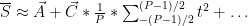
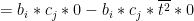
Let’s consider a small test case with 2 sensors and 7 readings (N=2 and P=7).

$\mathbf{M} = 4*\begin{bmatrix} b_0^2 & b_0b_1 \\ b_0b_1 & b_1^2\end{bmatrix}$

If we start with a vector $v_0 = \begin{bmatrix} 1 \\ 1\end{bmatrix}$ then $||v_0|| = \sqrt{2}$ . On our first iteration we have:

$v_1 = \frac{4}{\sqrt{2}}\begin{bmatrix} b_0^2 & b_0b_1 \\ b_0b_1 & b_1^2\end{bmatrix}\begin{bmatrix} 1 \\ 1\end{bmatrix} = \begin{bmatrix} b_0^2 + b_0b_1 \\ b_0b_1 + b_1^2\end{bmatrix}$

Our scale factor becomes $||v_1|| = \sqrt{(b_0^2 + b_0b_1)^2 + (b_1^2 + b_0b_1)^2}=\sqrt{b_0^4+2b_0^3b_1+2b_0^2b_1^2+2b_0b_1^3+b_1^4}$ .

On each iteration, we get different combinations of power terms occurring, and a longer and longer scale factor. In simple 2×2 matrix examples I’ve seen it takes about 10 iterations to converge.

As the covariance matrix is symmetric, with a 2×2 example we only have differing terms on the diagonal. As we iterate using the power method, we have a number of terms that are shared by both vector elements and a number of terms that are not shared. The terms that are not shared influence how the vector changes over time, and these non-shared terms are increasingly influenced by the differing diagonal elements, while the scaling at each iteration stops explosion to infinity.

We can also see that P does not affect how the unit vector changes, it just sets an external scale factor. Also our time period does not really matter; what matters is the sampling rate over our time period. P only really matters for the accuracy of the approximation, which can be seen in the illustration above. A large value of P means that outer approximations (e.g. values of $t$ close to -(P-1)/2 and (P-1)/2) are less reliable, because we are moving further from our location of function approximation. This matches up nicely with the concept of local processing within the brain – “samples” in this sense may actually comprise physical objects (neurons and synapses) and so physicality limits the time resolution for function approximation – we need to be small and local.

Even with the simple 2×2 example above, we also see that there is no inherent pattern for the first eigenvalue – it’s direction depends on the relative values of $b_0$ and $b_1$ . Also, as we can always remove a scale factor, we do not need to worry about the absolute values of the coefficients, we can pick a scale range that works for us and that simplifies the calculations. For example, this could be a normalised range between 0 and 1 or integer values between 0 and 255 (for 8-bit computations). All we need to beware of is overflow when performing the calculations; however, the scaling brings us within a common range at every iteration, so we just need to worry about overflow within each iteration. For example, we could perform the iteration multiplications with 16-bit values and then convert back down to 8-bit values once the scaling is applied.

Swift Taylor Approximations

Sensors

Measured Functions