When researching the neo-cortex, and machine learning methods, I keep coming back to certain themes. This post looks at one of those: the power iteration method for principal component analysis.
Background
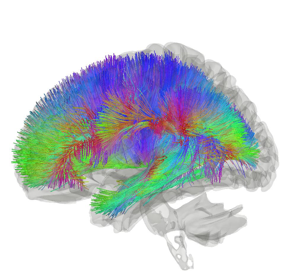
The neo-cortex has a particular pattern of connectivity with the thalamus. There are massive feedback circuits, and information flows appear to be duplicated in several places. This connectivity shows we have more than a simple input-output processing pipeline.
The neo-cortex appears to work in an unsupervised manner. It is performing some form of processing, but it has no access to a taught or “true” label. This differs from many popular machine learning methods that work in a supervised manner. In these latter cases, machine learning methods are working as classifiers, where the output of the classifier needs to be provided to train the classifier.
On the machine learning side, we only have a handful of methods for unsupervised learning. These include principal component analysis and factor analysis, clustering and graph-based approaches. The more you look into them the more you see the overlap between them, but for now we will concentrate on principal component analysis.
Dumb Biology
Biology is simple and dumb.
However, it is very good at stochastic repetition at scale.

This is good and bad. It is bad because at the higher levels of scale, say a human body, we have mind-boggling complexity. But it is also good, because it gives idiots like myself hope of understanding certain underlying processes that generate the complexity.
This raises the question: if the neo-cortex is implementing unsupervised machine learning methods in a “dumb” manner, how could this be achieved?
Simplicity & Repetition
To answer this question, we can ask another: what simple, repetitive methods are used in engineering to perform complex multi-dimensional unsupervised learning?
The answer is, surprisingly, not many.
Most engineering attempts require a large body of sunk knowledge. In these cases, the engineer needs to “play god” in relation to the system they are designing.
Principal component analysis is often dismissed for complex control and classification implementations due to several major disadvantages:
- it is very sensitive to scaling and so easy to bork;
- it is linear and so cannot capture most of the non-linear patterns in the real world; and
- it involves the eigendecomposition of large matrices, which is complicated and cannot be performed in real-time for very large matrices.
However, the power iteration method for performing principal component analysis caught my eye. While it doesn’t overcome the linearity problem, it does offer a relatively “dumb” approach to performing the eigendecomposition.
Power Iteration
The power iteration method is a rather obscure trick that is used to perform principal component analysis on large real-world datasets. It typically gets little coverage in academic engineering classes as it doesn’t lend itself to undergraduate teaching exercises. It is, however, widely used in industry. For example, it was used in Google’s early implementations of the PageRank algorithm.
How It Works
To apply the power iteration method, we start with an estimate of the covariance matrix.
Covariance Matrix & Mean Adjustment
Normally, it is recommended to use a mean-adjusted signal to construct the covariance matrix. This means subtracting a mean value of the signal from the original data points.
If we have a matrix X with measurements aligned as rows and dimensions of the data aligned as columns, we can compute a mean adjusted version of the matrix X’ by subtracting the mean across the rows from each row. We can then compute the covariance matrix as 
What is the data?
The “dimensions of the data” may be the values of a signal vector – e.g. a frequency spectrum with 256 data points across the frequency range of 0 to 20kHz has 256 “dimensions”. A 32 by 32 pixel image in greyscale flattened in a raster format along its rows has 1024 “dimensions”. Sometimes a “dimension” can be referred to as a data “element” as it corresponds to an element of the vector array (e.g. a location in a list of a set length).
“Measurements of the data” may be individual recordings of a signal. In many cases, a signal may be recorded over time, so the value of the signal vector at each time step may be a “measurement”. For example, a time sample of an audio recording or a frame of video may be a “measurement”.
Principal component analysis basically involves the decomposition of a covariance matrix for a set of data. The power iteration method is a way to perform this decomposition using the power of time and brute-force stupidity. I like it.
Iterating
The power iteration method is quite simple.
We start by taking a random unit vector – 
This vector is the same dimensionality or length as our signal, e.g. 256 for our frequency vector above. The vector is a “unit” vector as we scale the vector to have a predefined length, typically 1. Scaling the vector may involve dividing each element by the square root of the sum of the squares of the element values (i.e. the magnitude of the signal in the n-dimensional space or the L-2 norm).
The power iteration method then involves iteratively multiplying the random unit vector by the covariance matrix – 
The first stable vector value gives us our largest eigenvector. We can define “stable” in relation to a difference or distance between the old vector and the new vector.
Scaling
We can also divide by the magnitude of the vector to get a “unit” eigenvector – 
Deflation
To get the next eigenvector, we use a process called deflation. This involves modifying our original data using our first eigenvector, and then repeating the processing with the resulting signal.
I’ve found the online resources for deflation to be a bit patchy. There appear to be a few methods.
In one method, the first eigenvector 


Hotelling’s deflation is one of the earlier methods. However, several sources indicate this often suffers from problems and should be avoided. Preferred methods are a projection method or Wielandt’s Deflation (see pages 92-96). I like the projection method as it is more intuitive. A revised covariance matrix may be computed using 
Rayleigh’s Quotient
A variation of the power iteration method uses the Rayleigh Quotient. It is explained here. The unit vector 

The method is then iterated using the Quotient as opposed to the unit vector. This can allow for quicker convergence. It is basically a form of optimised scaling of the unit vector.
Online Principal Component Analysis
There are a few resources out there on “online PCA”. This turns out to involve methods similar to the deflation approaches set out above. These suggest a way that we can deflate eigenvector by eigenvector. This also turns out to have some interesting properties that are compatible with the wiring and organisation of the thalamus and neocortex.
Transforming Input Data
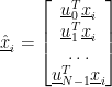
In conventional principal component analysis, the “components” or eigenvectors of the covariance matrix are typically returned as a matrix. This is sometimes called a transform matrix (e.g. in line with the “transform” operation in Scikit Learn). I’ve found that different libraries organise this differently, but let’s stick to the convention of Scikit Learn and consider this as having each eigenvector on each row and the features or dimensionality of the eigenvectors across the columns. (This tutorial organises the matrix with the eigenvectors as columns of 
Many use
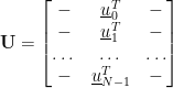
Where there are N components or eigenvectors and:

I.e 
In this case, we can use the transform matrix
And where:

Back to Deflation
Now, when we use deflation projection, we find the components or eigenvectors one-by-one. The original data is first projected onto a basis formed by the first component or eigenvector to generate adjusted data. The power iteration may then be applied to the adjusted data to find the next eigenvector. This also appears to form the basis for most online principal component analysis methods.
Many deflation methods concentrate more on adjustment of the covariance matrix. For example, the projection deflation method set out above adjusts a convariance matrix as follows

Where:
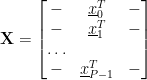
I.e. the rows are the different data samples, where there are P data samples, and the columns are the data features.
In the above equation for 


Now for online methods, we don’t necessarily have a set of input data in matrix form. 


Hence, we have a method for adjusting incoming data samples: we multiply them (project) using
Adjusting Individual Data Samples
Let’s return to the Scikit Learn formulation of the transform operation: 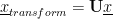


In Euclidean space, the projection 

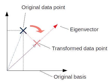
In two dimensions, 


Now, in our deflation methods we were computing 

Relating Deflation and Projection
It turns out we can.
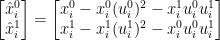
Let’s consider the deflation projection performed for 1 data sample (i.e. P =1) using a general component or eigenvector
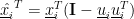
Let’s then consider a two-dimensional example so that we can zoom into the individual vector elements:


So, rearranging into column vectors for clarity:
Now if we look at the projection 

This looks familiar. If we then compute 

I.e. the same expression as if we started from the deflation projection.
This is all a long-winded way of saying that, once we have a first component or eigenvector, we can adjust our original data by subtracting the projection of the original data onto the component or eigenvector, as represented in the basis space of the original data. We can then repeat the power iteration process on the adjusted data to get a second component or eigenvector.
Very Interesting
The “adjustment” to the original data is very interesting. There are a number of different ways of looking at it, and each way provides a different insight into how this may be implemented using simple biological structures. Each way also links with a different approach taken in the machine learning literature.
The transform for principal component analysis is sometimes used in machine learning to attempt to decorrelate input data. For example, Geoff Hinton refers to this in slide 13 of these lecture notes. The transform is typically applied in the matrix form above, i.e.
The traditional application of the transform for principal component analysis computes the projection of the original data onto different components or eigenvectors. For example, a first element in 


Now one benefit of principal component analysis is that the eigenvectors are orthogonal. This means that 

Now, it’s interesting to consider the full pipeline involving the inverse transform:

Now normally we wouldn’t look too closely at 
Considering again a simple two-dimensional case where 

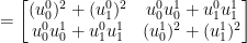
The result is a F by F matrix can be used to transform a data sample:


Now this appears to equal:

(Aside: I need to look into this in more detail – I think there may be terms that relate to 

So we can see that when we compute
Feed Forward and Feed Back
Considering the methods above, we can see the sketchy outline of feed forward and feed back data pathways.
We first compute a first component or eigenvector 
In a feed forward direction, we compute a transformed element using the first component or eigenvector 
In a feed back direction, we adjust our original data to remove a contribution in the direction of the first component or eigenvector
We can then repeat this process with diminishing returns for each subsequent component or eigenvector up to the dimensionality of our original data.
The feed back adjustment has an additional advantage. It allows us to determine whether we actually need to make another iteration of the complete process to determine the next component or eigenvector. For example, we can look at the magnitude of the adjusted data sample. If it is below a threshold we can stop the method and just use our existing elements.
Back to the Cortex
The iterative methods discussed above lend themselves to the wealth of sensory information that even simple brains experience every day. You can see how they could be implemented by just passing signals through a slowly changing structure.
The deflation methods also seem to sync with the feedback connections to the thalamus. They suggest that the cortex is applying a common processing approach to different sensory signals where this approach requires repeated modification of incoming signals.
In power iteration methods, a direction of largest variation is first determined. This seems sensible from an evolutionary perspective, we want our brains to determine the core axes of variation in our world first, as these will likely have the biggest impact, and are easiest to detect. We can then look for more subtle variance in the world. This offers diminishing returns and the power iteration method allows us to stop when we cease to receive useful signals.
