Analysing Your Tweets with ChatGPT

This post dives into applying ChatGPT’s new Code Interpreter / Advanced Data Analysis to downloaded Twitter data. Keep reading for an insight into the cool things you can do.

If you want to just skip to some function code see here.

Advanced Data Analysis

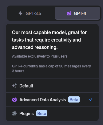
The Advanced Data Analysis option in (paid-for) ChatGPT is a sandboxed code execution environment that allows file uploads and downloads. This means you can run code in the chat. This is very useful for data analysis. You can run common scikit learn code and display the results using matplotlib. You can select the Advanced Data Analysis mode when selecting the model at the top of a new chat:

Twitter Archive

Until Elon Musk purposefully tanked the platform, I used Twitter as a notebook for random thoughts and insights. This is better than a notebook because I can also (currently) access all my Twitter data as a downloadable archive. This data provides a fascinating experimental dataset for data analysis. (Yes, it’s a bit navel-gazing but you cannot easily get data for multiple users through the Twitter API, so your own data is the best data source you have.)

To get your Twitter data, go to “More” in the left-hand menu, then “Your Account”, then “Download an archive of your data”. You’ll be prompted for your password and then archiving will be scheduled. A little later (e.g., a day or two), you’ll receive an email with a link to download the archive as a ZIP file. My archive was around 250MB so make sure you download over a fast internet connection!

The archive has the following structure:

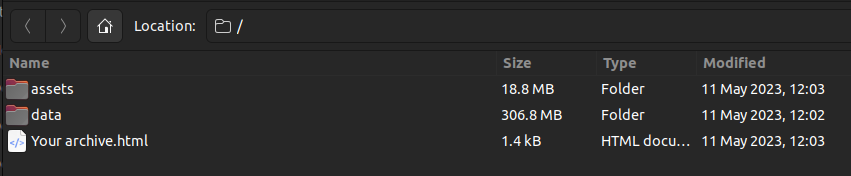
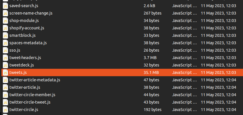
The data folder contains all your Twitter data as JSON files. There’s a lot in here and all your posted media is also included. For this analysis we will just use the tweets.js file within the data folder. This contains the actual tweet data (without associated media). It is also a reasonable size. My file contained data for around 23,436 tweets.

Playing Around

I started by just naively uploading the tweets.js file and asking ChatGPT to analyse it.

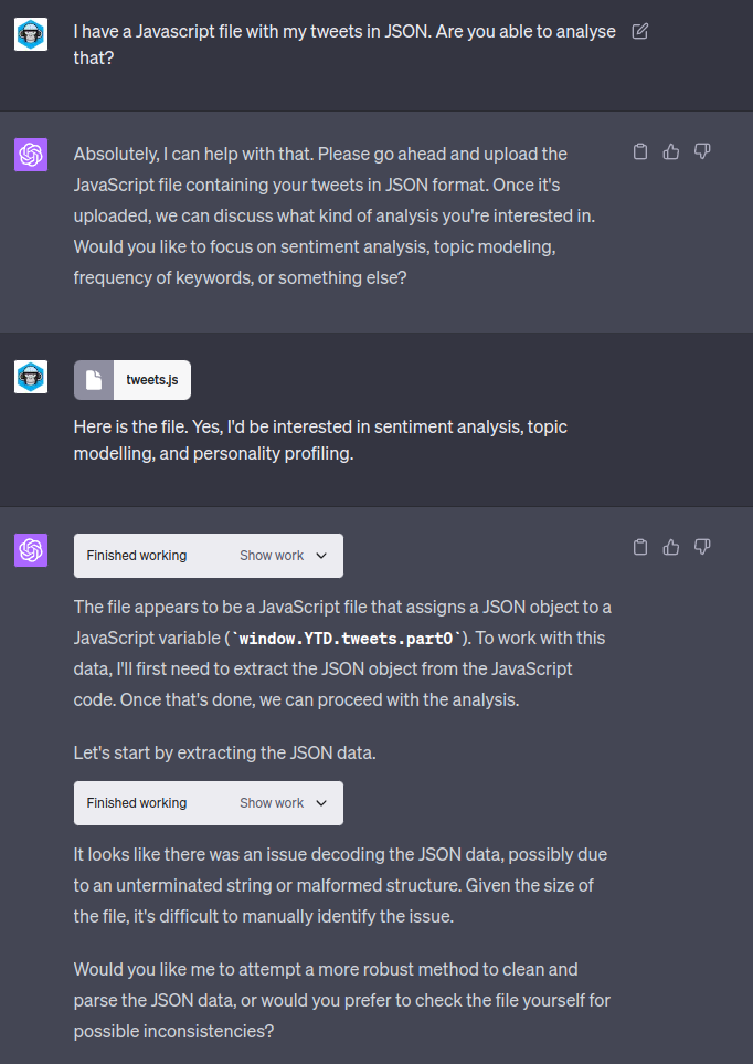
As you can see, ChatGPT had an issue naively parsing the JSON file. However, this wasn’t my first rodeo – I knew that the variable definition in the JSON caused issues with the load from previous experiments. What is very cool and somewhat weird is being able to just tell ChatGPT what you think the solution might be and that is enough to generate working code!

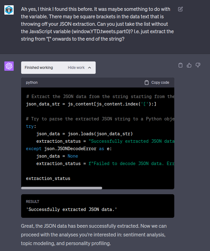
If anyone has an issue parsing the tweets.js file, the trick is the code below, which extracts from the first [ to the end of the file:

import json

# First, let's read the content of the uploaded JavaScript file to see its structure.
file_path = '/mnt/data/tweets.js'

# Read the file content
with open(file_path, 'r', encoding='utf-8') as f:
    js_content = f.read()

# Extract the JSON data from the string starting from the first square bracket '[' to the end of the string
json_data_str = js_content[js_content.index('['):]

# Try to parse the extracted JSON string to a Python object
try:
    json_data = json.loads(json_data_str)
    extraction_status = "Successfully extracted JSON data."
except json.JSONDecodeError as e:
    json_data = None
    extraction_status = f"Failed to decode JSON data. Error: {e}"

extraction_status

Analysis

Based on some back-and-forth with ChatGPT, I decided to start by looking at sentiment analysis, topic modelling, and personality profiling.

As a caveat, much of the analysis is somewhat crude and simplified – think undergraduate coding exercises or online tutorial level. But they do provide a nice baseline of “this is the known starting point” for you to explore more deeply. The best way to use ChatGPT is to start with the most likely, view that, and then to iterate into more original space.

Sentiment Analysis

I was amazed by how easy it is to do this – I just asked!

ChatGPT uses a known Python library called TextBlob to perform the analysis – it writes then runs the code and displays the output!

Topic Modelling

ChatGPT suggested LDA to perform topic modelling. This gave me confidence as I have a long history using Gensim to perform LDA in the pre-neural network days. (I was never much enamoured with LDA – the results seemed very token form dependent – the new sunny uplands of vector embeddings are much better.)

I did run into a problem as ChatGPT was using the nltk stopwords but you have to download these first. ChatGPT said it wasn’t capable of doing that so it constructed a set of stopwords from scratch. Again, this shows that you have to know what you are doing a little to get the best out of ChatGPT.

Another warning: ChatGPT is sometimes an unreliable narrator. It would often say “I cannot run this code because X” and I would look at the error message and it would actually be because of Y. If you then steer ChatGPT to fix Y, things would work. If you let ChatGPT fix the error itself, it would often be lost down rabbit-holes trying to fix non-error X.

With the topic modelling, we iterated a few times to improve the tokenisation and stopwords. Concatenations (“‘t”, “‘s”) and “&” as HTML encoded seemed to throw off the modelling. Asking ChatGPT to add to the stopwords and tweak the data cleaning worked well:

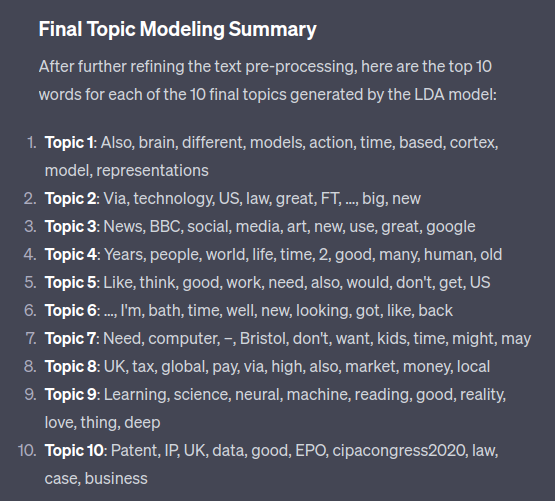
Here is a plot of the word weighting in each topic:

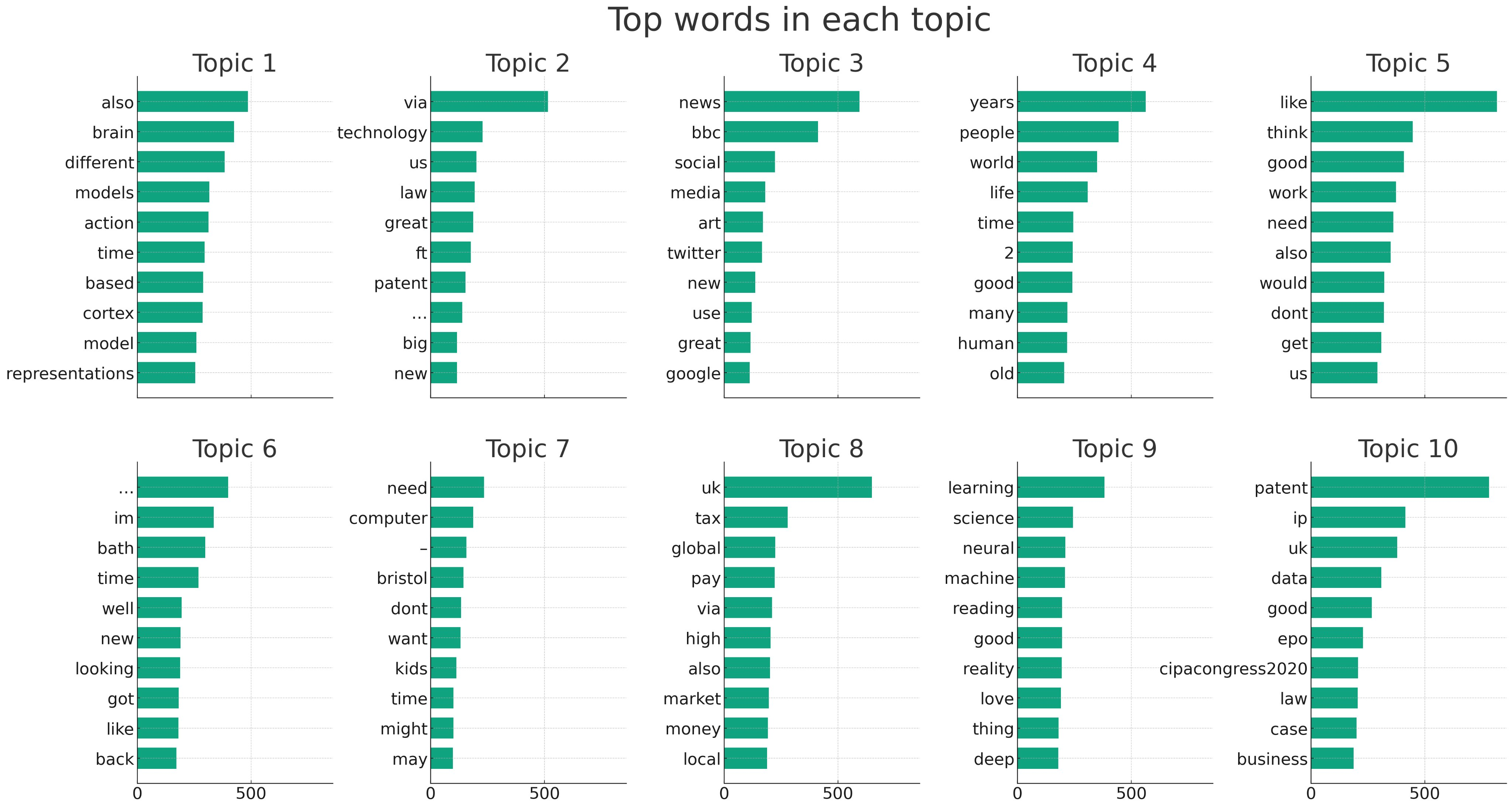
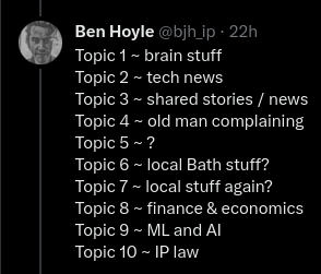
And this was ChatGPT’s analysis:

I was impressed with ChatGPT’s analysis here – before this output I’d had my own guess and the two align well:

Personality Profiling

From my chats with ChatGPT I know it’s really into the “Big Five” personality traits. It must be all that imbibed tech bro chat and corporate bullshit (it’s okay as a rough model and there is some alignment to actual human traits but it can also be a lot of horoscope-style woo dressed up as science). Here was no exception:

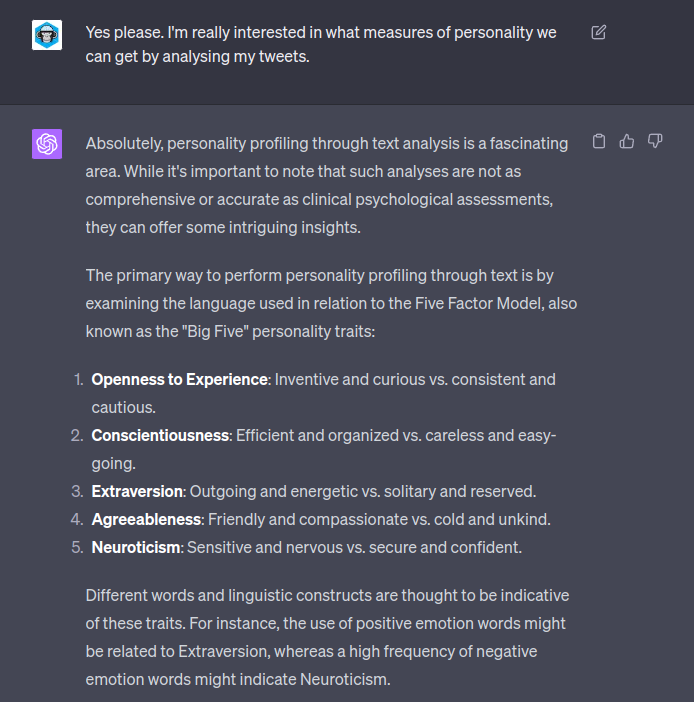
ChatGPT’s approach here was very simple. It just looked for keyword matches in the text.

# Define lists of words associated with each Big Five personality trait
# These are simplified and illustrative; more comprehensive dictionaries are typically used in research
openness_words = ['creative', 'curious', 'imaginative', 'insightful', 'original', 'wide interests', 'artistic', 'intelligent']
conscientiousness_words = ['organized', 'reliable', 'dependable', 'ambitious', 'disciplined', 'dutiful']
extraversion_words = ['active', 'assertive', 'energetic', 'outgoing', 'talkative', 'engaged']
agreeableness_words = ['appreciative', 'kind', 'generous', 'sympathetic', 'trusting', 'warm', 'compassionate', 'considerate']
neuroticism_words = ['anxious', 'self-pitying', 'tense', 'moody', 'emotional', 'jealous', 'envious']

I don’t really think this has much utility, and is firmly within the ballpark of bullshit pseudo-science methods associated with the “Big Five”. But let’s give it a whirl.

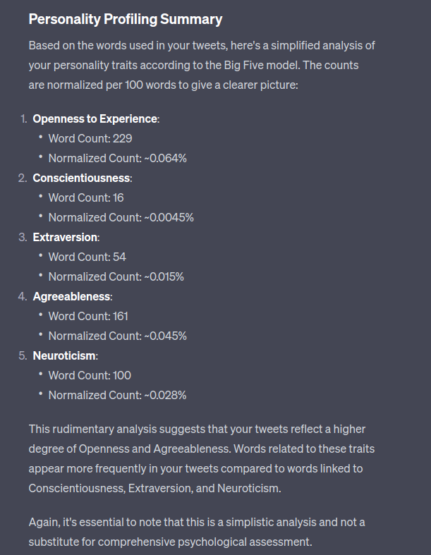
Fair play to ChatGPT – it does call out it’s own simplicity. This would maybe be a good starting point for a much better and deeper analysis. For example, you could use spaCy to provide improved tokenisation and parsing and you could use a vector-based method of word similarity.

I tried to get ChatGPT to deepen the analysis but it ended up performing more keyword matching:

Again, the analysis seemed better, but I have a sneaking suspicion ChatGPT is telling me what I want to hear based on my custom system prompt:

Embeddings

I tried to ask ChatGPT to do some analysis based on vector embeddings. It turns out this is a step too far for the sandbox environment (fair play).

In my experience, all of these pre-neural approaches are a bit rubbish. I like it when you can have a friend / work colleague agree with you on that:

I suggested I run some embeddings locally and upload these for ChatGPT to play with.

A cool feature of the Advanced Data Analysis mode is you can get ChatGPT to do the pre-processing and file saving for you, and write the scripts to load the data locally! Even though I can do this myself, I am lazy and it is great to offload this banal work to the robots.

Another warning: always check the code and file in a safe sandboxed environment before running locally. I prefer copy-and-pasting code because I can then see what the code is and what it is doing.

I steered ChatGPT towards the excellent and now-defacto-industry-standard SentenceTransfomer library for performing the embeddings (all the cool VC funded vector database companies tend to be using this under the hood). ChatGPT chose the paraphrase-MiniLM-L6-v2 model by default but I prefer the slightly larger and better all-MiniLM-L6-v2.

from sentence_transformers import SentenceTransformer
import pickle
import json

# Load the tweets from the pickle file
with open('tweets_text.pkl', 'rb') as f:
    tweets = pickle.load(f)

# Initialize the sentence transformer model
# You can choose a specific model from: https://www.sbert.net/docs/pretrained_models.html
model = SentenceTransformer('paraphrase-MiniLM-L6-v2')

# Generate embeddings for each tweet
embeddings = model.encode(tweets)

# Create a dictionary to hold the tweet and its corresponding embedding
tweet_embeddings = {tweet: embedding.tolist() for tweet, embedding in zip(tweets, embeddings)}

# Save the tweet and embeddings as a JSON file
with open('tweet_embeddings.json', 'w') as f:
    json.dump(tweet_embeddings, f)

print("Tweet embeddings have been saved to 'tweet_embeddings.json'")

For nearly 25,000 tweets the embedding file is near 200MB. This starting breaking the sandbox, causing memory issues and other glitches:

ChatGPT was sometimes a little too optimistic on iterative fixes and you can easily get trapped in sink holes of patches and non-working code. I steered ChatGPT to the more efficient compressed numpy .npz file type, which was ~40MB.

ChatGPT had lots of good ideas about clustering with scikit-learn and projection with t-SNE (two of my “go-to” exploration methods). But we couldn’t get these working in the sandbox environment, so we had to move to my more powerful local GPU machine.

What I like about ChatGPT is you can seamlessly move from beginner to more advanced methods without blinking.

So I ran these locally, which took a minute or two. No clear “k” value for the number of clusters jumped out, but the silhouette analysis appeared to plateau out after ~10 clusters.

We also tried some PCA dimensionality reduction on the embeddings. This produced some cool power law curves:

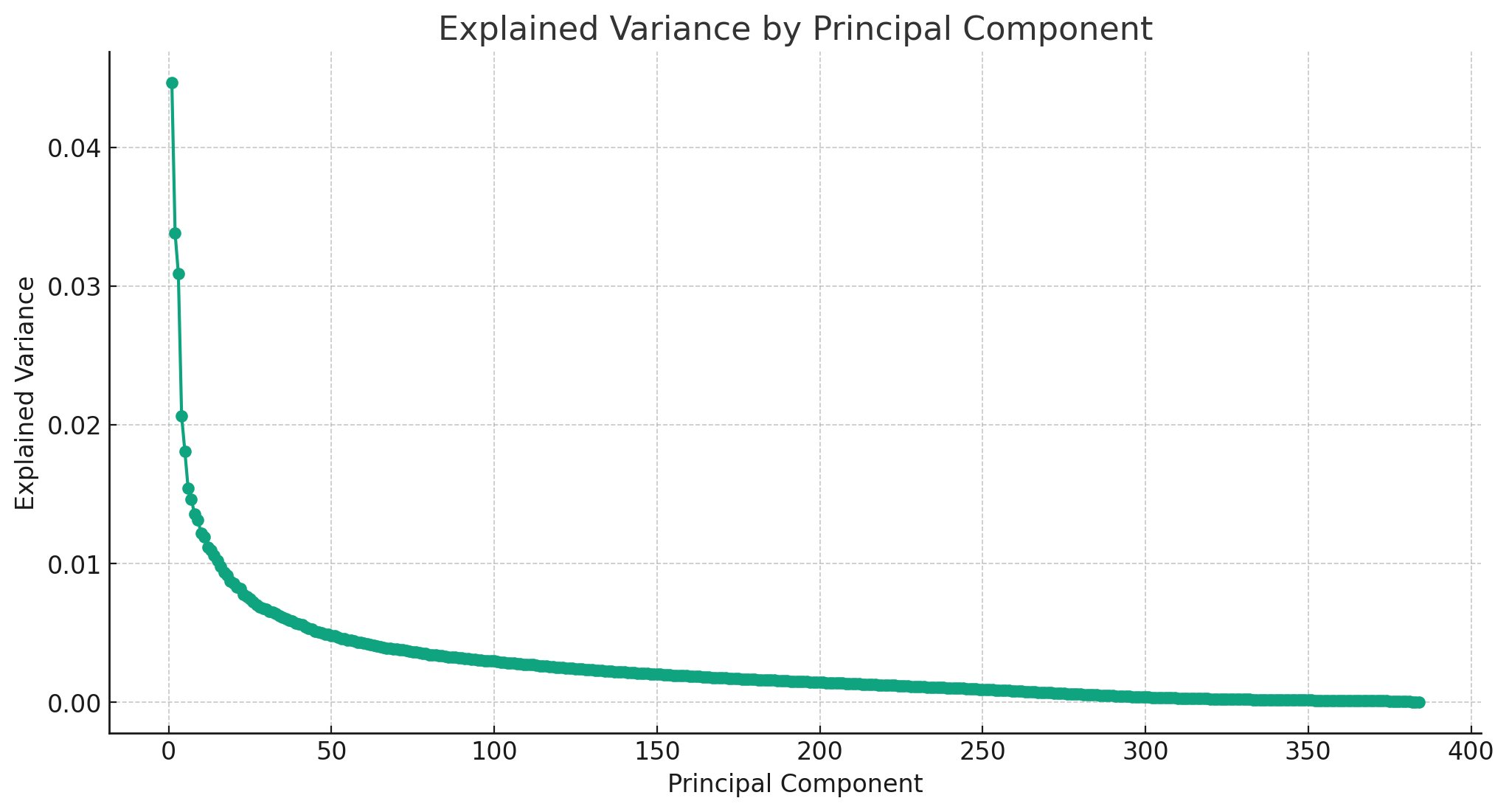
A large amount of the variance can be explained with a handful of components, but lifelike detail requires a long tail of small additions. This pattern can be found with many things.

Tweet Vector Database Query

Once we encoded the tweets with the SentenceTansformer, it was easy to put together a simple script to run a vector query on the tweet archive.

import numpy as np
from sklearn.metrics.pairwise import cosine_similarity
from sentence_transformers import SentenceTransformer
import textwrap

# Load pre-trained sentence transformer model
model = SentenceTransformer('all-MiniLM-L6-v2')

# Load tweet embeddings and texts
data = np.load('tweet_embeddings.npz')
tweet_texts = data['texts']
tweet_embeddings = data['embeddings']

# Get user input for query text and number of results
query_text = input("Enter the query text: ")
num_results = int(input("Enter the number of results to return: "))

# Encode the query text
query_vector = model.encode([query_text])
query_vector = query_vector.reshape(1, -1)

# Compute cosine similarities
similarities = cosine_similarity(query_vector, tweet_embeddings)

# Sort by similarity
sorted_indices = np.argsort(-similarities[0])

# Print top N most similar tweets
print(f"Top {num_results} most similar tweets to '{query_text}':")
for i in range(num_results):
    index = sorted_indices[i]
    wrapped_text = textwrap.fill(tweet_texts[index], width=200)
    print(f"{i + 1}. {wrapped_text}\n(Similarity: {similarities[0][index]:.4f})\n")

This works well:

My experience with vector search is that it doesn’t really matter what the encoding is (I’ve had good results from the all-MiniLM-L6-v2 model and using OpenAI’s ada embeddings). The results are great and much better than traditional keyword search.

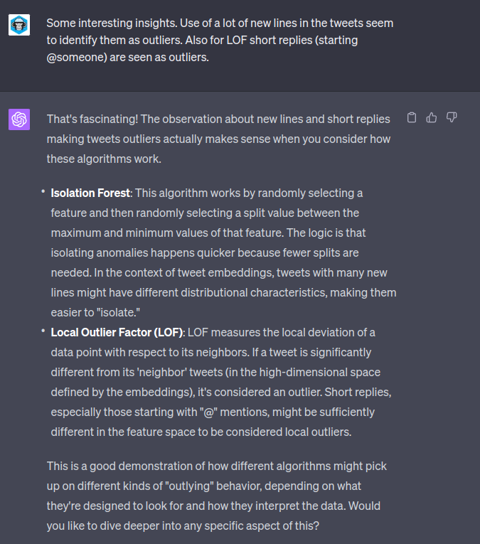
Outlier Analysis

We also had a play with outlier analysis:

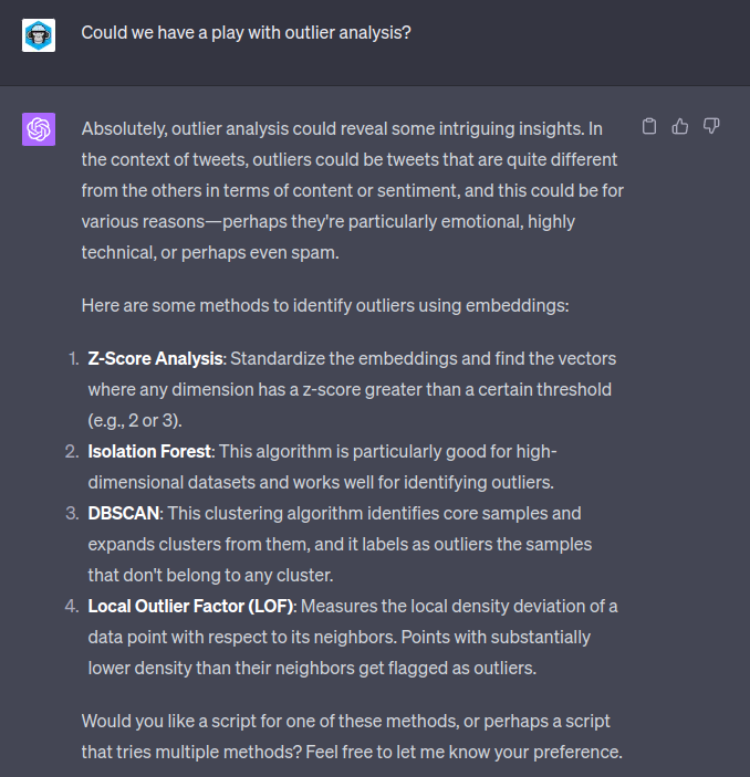
This seemed a little ropey with the returned data. It seemed to be led a lot by the surface form of the text – tweets with newlines or “@replies” seemed to be often classed as “outliers”:

More Clustering

I like to use the Python plotly library for clustering. You get some lovely Javascript webpages that you can explore with hover-over.

import numpy as np
import plotly.express as px
from sklearn.cluster import KMeans
from sklearn.manifold import TSNE
from sklearn.preprocessing import StandardScaler

# Load embeddings and texts from npz file
loaded = np.load('tweet_embeddings.npz', allow_pickle=True)
embeddings = loaded['embeddings']
texts = loaded['texts']

# Step 1: Standardize the data
scaler = StandardScaler()
scaled_embeddings = scaler.fit_transform(embeddings)

# Step 2: Perform clustering (here using KMeans, you can replace with other algorithms)
n_clusters = int(input("Enter the number of clusters: "))  # You can change the number of clusters
kmeans = KMeans(n_clusters=n_clusters, random_state=0).fit(scaled_embeddings)
labels = kmeans.labels_

# Step 3: Dimensionality reduction using t-SNE
tsne = TSNE(n_components=2, random_state=0)
reduced_embeddings = tsne.fit_transform(scaled_embeddings)

# Step 4: Create Plotly visualization
df = {
    'x': reduced_embeddings[:, 0],
    'y': reduced_embeddings[:, 1],
    'labels': labels,
    'texts': texts
}

fig = px.scatter(df, x='x', y='y', color='labels', hover_data=['texts'])
fig.show()

Unfortunately, you can’t explore the text via hoover-over in the PNG below. This is a case with 10 clusters:

As a rough guide to the clusters:

• Top left blue is patents.
• Surrounding yellow is case law.
• Left-hand-side purple is politics.
• Centre orange is short replies and retweets.
• Top peach is computing.
• Purple to the right of that is neural nets.
• Darker purple on far left is neuroscience.
• Middle adjacent blue/purple is “life” and philosophy.
• Centre fuchsia is sociology.
• Bottom left orangey-peach is music.
• Upper left above politics purple is economics light orange.

What I love about embedding clustering, which you don’t get with LDA, is that the groupings seem intuitive and reasonable.

Here are six clusters:

This is me in a nutshell:

• Purple – IP law
• Peach – politics and economics
• Yellow – replies, and culture (music, film, art etc)
• Orange – life and philosophy
• Fuchsia – neuroscience
• Dark blue – technology

Time Analysis

We also did some cool local analysis looking at time-series aspects.

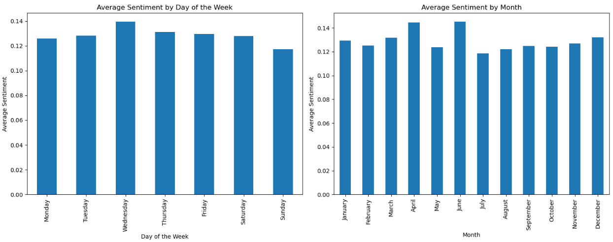
This uses the cool group-by functionality of pandas:

import json
from textblob import TextBlob
import matplotlib.pyplot as plt
import pandas as pd
from datetime import datetime

# Load tweets from the JSON file
with open("tweets.js", "r") as f:
    data_str = f.read()[len("window.YTD.tweet.part0 = "):]
    tweets_data = json.loads(data_str)

# Extract tweet texts and created_at fields
tweets = [(tweet['tweet']['created_at'], tweet['tweet']['full_text']) for tweet in tweets_data]

# Convert to DataFrame for easier manipulation
df = pd.DataFrame(tweets, columns=['created_at', 'text'])

# Convert 'created_at' to datetime format and extract day and month
df['created_at'] = pd.to_datetime(df['created_at'])
df['day_of_week'] = df['created_at'].dt.day_name()
df['month'] = df['created_at'].dt.month_name()

# Calculate sentiment scores
df['sentiment'] = df['text'].apply(lambda x: TextBlob(x).sentiment.polarity)

# Group by day of the week and month, then calculate mean sentiment
df_by_day = df.groupby('day_of_week')['sentiment'].mean().reindex([
    'Monday', 'Tuesday', 'Wednesday', 'Thursday', 'Friday', 'Saturday', 'Sunday'])
df_by_month = df.groupby('month')['sentiment'].mean().reindex([
    'January', 'February', 'March', 'April', 'May', 'June',
    'July', 'August', 'September', 'October', 'November', 'December'])

# Plotting
plt.figure(figsize=(15, 6))
plt.subplot(1, 2, 1)
plt.title('Average Sentiment by Day of the Week')
df_by_day.plot(kind='bar')
plt.xlabel('Day of the Week')
plt.ylabel('Average Sentiment')

plt.subplot(1, 2, 2)
plt.title('Average Sentiment by Month')
df_by_month.plot(kind='bar')
plt.xlabel('Month')
plt.ylabel('Average Sentiment')

plt.tight_layout()
plt.show()

Final Thoughts

I was very impressed by the inbuilt abilities for data science. You can easily do advanced data analysis by just dropping in a reasonably sized CSV or Excel file. It definitely speeds things up by a factor of 5-10x to be able to just run the code and see the graphs, rather than implement locally by hand. Any small business or university researcher can now ask complex data-driven questions without needing any special skills (apart from a GPT-4 subscription).

Existing data scientists need not despair. They have the skills to quickly check “default” methods and to rapidly explore and test more advanced analysis. Everyone will win.

Having the ability to copy and run small scripts locally on a more powerful GPU machine is definitely useful if you have bigger datasets or need to do things with higher dimensionality data, such as text-as-embeddings or images.

Some of the code for the local functions is available on GitHub here.