Bio-Inspired Robotics for Beginners

There are several well-known problems with modern “deep” learning approaches. These include the need for large quantities of training data and a lack of robustness. These are related. Neural network architectures are trained by computing an error between some “ground truth” data in the training data and the architecture’s prediction of that same data, given a set of associated input data. The error is directed based on differentials for each component of the architecture. This feels to me as doing everything in reverse.

Animal brains offer an alternative view of intelligence. Animals are not taught complex behaviours by providing millions of labelled training examples. Instead, they learn the natural (local) structure of their environment over time.

What Do We Know that Might Help?

So, what do we know about animal brains that could help us build artificial intelligent systems?

Quite a lot it turns out.

Mammals have evolved a clever solution to the problem of predicting their environment. They have multiple sense organs that provide information in the form of electrical signals. These electrical signals are provided to neural structures. There are roughly three tiers: the brainstem, the midbrain and the cortex. These represent different levels of processing. They also show us the pathway of evolution: newer structures have been built on top of older structures, and older structures have been co-opted to provide important support functions for the newer structures.

In the mammalian brain there are some commonalities as to how information is received and processed. The cortex appears to be the main computational device. Different sensory modalities appear to be processed using similar cortical processes. Pre-processing and feedback is controlled by the mid-brain structures such as the thalamus and basal ganglia.  

In terms of knowledge of sensory processing, we know most about the visual system. We then know similar amounts about auditory and motor systems, including perception of the muscles and skin (somatosensory). We know the least about smell and interoception, our sensing of internal signals relating to organs and keeping our body in balance. All the sensory systems use nerve fibres to communicate information in the form of electrical signals.

Cortex I/O

In mammalian brains, the patterns of sensory input to the brain and motor output are fairly well conserved across species. All input and output (apart from smell) is routed via the thalamus. The basal ganglia appears to be a support structure for at least motor control. The brain is split into two halves, and each half receives input from one side of the body. Most mammals have the following:

• V1 – the primary visual cortex – an area of the cortex that receives an input from the eye (the retina) via the thalamus;
• A1 – the primary audio cortex – an area of the cortex that receives an input from the ear via the thalamus;
• S1 – the primary somatosensory cortex – an area of the cortex that receives an input from touch, position, pain and temperature sensors that are positioned over the skin and within muscle structures (again via the thalamus);
• Insula – an area of the cortex that receives an input from the body, indicating its internal state, from the thalamus; and
• M1 – the primary motor cortex – an area of the cortex that provides an output to the muscles (it receives feedback from the thalamus and basal ganglia).

For a robotic device, we normally have access to the following:

• Image data – for video, frames (two-dimensional matrices) at a certain resolution (e.g. 640 by 480) with a certain frame rate (e.g. 30-60 frames per second) and a certain number of channels (e.g. 3 for RGB). The cortex receives image information via the lateral geniculate nucleus (LGN) of the thalamus. The image information is split down the centre, so each hemisphere receives one half of the visual field.  The LGN has been shown to perform a Difference Of Gaussians (DOG) computation to provide something similar to an edge image. The image that is formed in M1 of the cortex is also mapped to a polar representation, with axes representing an angle of rotation and a radius (or visual degree from the horizontal).
• Audio – in one form, a one-dimensional array of intensities or amplitudes (typically 44100 samples per second) with two channels (e.g. left and right). The cochlea of the ear actually outputs frequency information as opposed to raw sound (e.g. pressure) information. This can be approximated in a robotic device by taking the Fast Fourier Transform to get a one-dimensional array of frequencies and amplitudes. 
• Touch sensors / motor positions / capacitive or resistive touch – this is more ropey and has a variety of formats. We can normally pre-process to a position (in 2 or 3 dimensions) and an intensity. This could be multiple channel, e.g. at each position we could have a temperature reading and a pressure reading. On a LEGO Mindstorms ev3 robot, we have a Motor class that provides information such as the current position of a motor in pulses of the rotary encoder, the current motor speed, whether the motor is running and certain motor parameters. 
• Computing device information – this is again more of a jump. An equivalent of interoception could be seen as information on running processes and system utilization. If the robotic device has a battery this could also include battery voltages and currents. In Python, we can use something like psutil to get some of this information. On a LEGO Mindstorms ev3 robot, we have PowerSupply classes that provide information on the battery power.
• Motor commands – robotic devices may have one or more linear or rotary motors. Typically, these are controlled by sending motor commands. This may be to move to a particular relative position, to move at a given speed for a given time and/or to rotate by a given number of rotations.

We will leave smell for now (although it’s a large part of many mammals sensory repertoire). It probably slots in best as part of interoception. One day sensors may provide an equivalent data stream. 

We can summarise this rough mapping as follows:

Brain	Robot
Eyes / Retina > V1	Video Camera > Split L/R > Polar Mapping
Ears / Cochlea > A1	Microphone > Channel Split L/R > FFT
Outer body + muscle > S1	Multisensor > Position + value
Interoception > Insula	Device measurements > numeric array
M1 > muscles	Numeric commands > motors

One advantage of the “deep” learning movement is that it is now conventional to represent all information as multidimensional arrays, such as Numpy arrays within Python. Indeed, we can consider “intelligence” as a series of transformations between different multidimensional arrays.

Cortex Properties 

The mammalian cortex is a two-dimensional sheet. This provides a strong constraint on the computational architecture. Human brains appear wrinkly because they are trapped within our skulls and need to maximise their surface area. Mouse brains are quite smooth.

The cortex is a layered structure, providing its thickness. Each layer is a few mm in height. There are between 4 and 6 layers, depending on the area of the cortex. The layers contain a large number of implementing neurons. These neurons provide a combination of excitatory and inhibitory connections. Different layers receive different inputs and provide different outputs. Feedback appears to be supplied over a large area via layer 1, input is received from the thalamus at layer 4, input is received from other parts of the cortex at layers 3 and 4, layer 2 provides feed back to a neighbouring cortical area, layer 3 provides a feed forward output to other cortical areas (wider range) and layers 5 and 6 provide feedback to the thalamus, layer 5 also provides a feed forward output to a neighbouring cortical area. Computation occurs vertically in the layers and information is passed within the plane of the cortical sheet.

The two-dimensional cortical sheet of many mammals appears to have a common general topology. The input and output areas appear reasonably fixed, and are likely genetically determined.  The visual, somatosensory and motor areas appear aligned. This may be what creates “embodied” intelligence; we think conceptually using a common co-ordinate system. For example, the half an image from the eyes is aligned bottom-to-top within the visual processing areas, which is aligned with the feet-to-head axis of the body as felt and the feet-to-head axis of the body as acted-upon (i.e. V1, S1 and M1 are aligned). This makes sense – it is more efficient to arrange our maps in this way.

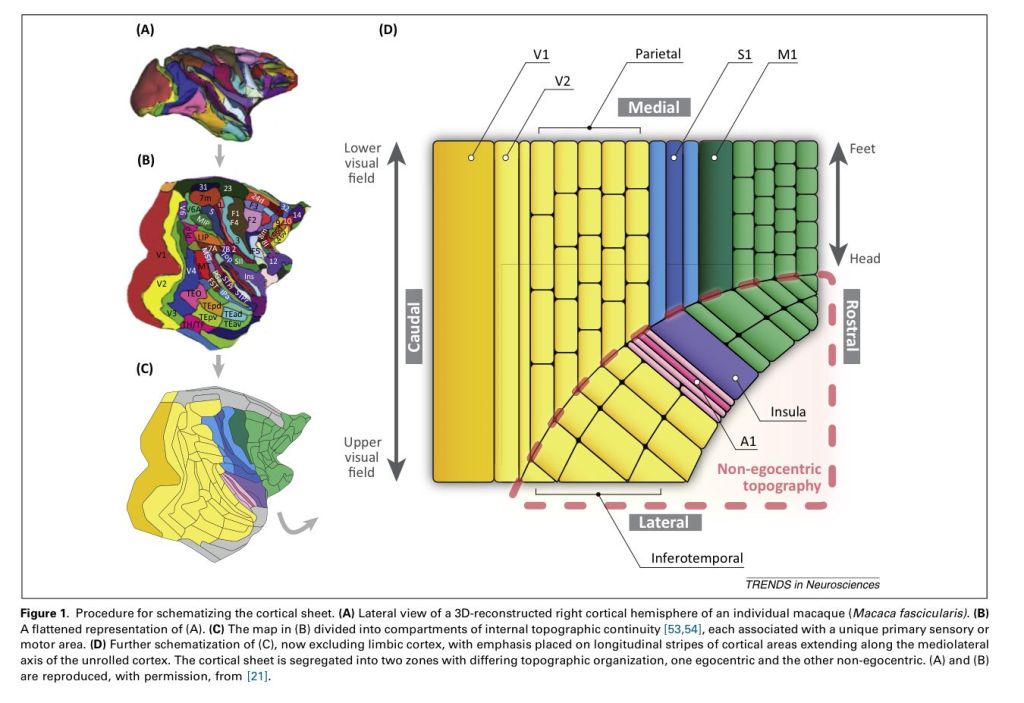
The cortex also appears to have neuronal groupings that have certain functional roles. This is best understood in the visual processing areas, where different cortical columns are found to relate to different portions of the visual field; each column has a receptive field equivalent to a small group of pixels (say somewhere around 1000). Outside of the visual field evidence is more shaky. 

The cortex of higher mammals also appears to have a uniform volume but a differing neuronal density. This neuronal density appears similar to a diffusion gradient. Within the visual areas towards the back of the brain there are a large number of neurons per square millimetre; towards the front of the brain there are fewer neurons per square millimetre. The baboon has a 4:1 ratio. However, because the volume of the cortical sheet is reasonably constant, the neurons towards the front of the brain are more densely connected (as there is room). A simple gradient in neuron number may provide an information bottleneck that forces a compression of neural representations, leading to greater abstraction.

Considering a two-dimensional computing sheet gives us an insight into two cortical pathways that have been described for vision. A first processing pathway (the dorsal stream) is the line drawn from V1 to S1 and M1. This pathway is swayed towards motion, i.e. information that is useful for muscle control. A second pathway (the ventral stream) is the line drawn from V1 to A1. This pathway is swayed towards object recognition, which makes sense because we can correlate audio and visual representations of objects to identify them. What is also interesting is that the lower visual field abuts the first processing pathway and the upper visual field abuts the second processing pathway – this may reflect the fact that the body is orientated below the horizontal line of vision and so it makes sense to map the lower visual field to the body in a more one-to-one manner.

The cortical sheet also gives us an insight into implementing efficient motor control. You will see that S1, the primary somatosensory area, is adjacent to M1, the primary motor cortex. This means that activation of the motor cortex, e.g. to move muscles, will activate the somatosensory representations regardless of any somatosensory input from the thalamus. We thus have two ways of activating the body representations, one being generated from the motor commands and one being generated by the input from the body. This gives us the possibility to compare and integrate these signals in time to provide control. For example, if the signal received from the body did not match the proposed representation from the motor commands then either the motor commands may be modified or our sensing of our body is modified (or both).

So to recap:

• the main computing machinery of the brain is a two-dimensional sheet;
• it has an embodied organisation – the relative placement of processing areas has functional relevance;
• it has a density gradient that is aligned with the embodied organisation; and
• it appears to use common, repeated computing units.

Cortex to Robot

This suggests a plan for organising computation for a robotic device.
Computers typically work according to a one-dimensional representation: data in memory. If we are creating a bio-inspired robotic device, we need to extend this to two dimensions, where the two dimensions indicate an ordering of processing units. It might be easier to image a football field of interconnected electronic calculators.

We can then align our input arrays with the processing units. At input and output areas of any computing architecture there could be a one-to-one organisation of array values to processing units. The number of processing units may decrease along an axis of the two-dimensional representation, while their interconnections increase. In fact, a general pattern is that connectivity is local at points of input or output but becomes global in between these points. These spaces in between store more abstract representations.

This architecture of the cortex reminds us of another architecture that has developed with “deep” learning: the autoencoder.

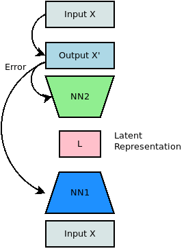
Indeed, this is not by accident – the structure of the visual processing areas of the brain has been the inspiration for these kind of structures. Taking a two-dimensional view of computation also allows us to visualise connectivity using a two-dimensional graph structure.

Onward!

So we can start our bio-inspired robot by constructing a setup where different sensory modalities are converted into Numpy arrays and then processed so that we can compare them in a two-dimensional structure. The picture becomes murkier once we look at how associations are formed and how the thalamus comes into the equation. However, by looking at possible forms of our signals in a common processing environment we can begin to join the dots.

References

• Barbara L. Finlay and Ryutaro Uchiyama. “Developmental mechanisms channeling cortical evolution.” Trends in neurosciences 38.2 (2015): 69-76.
• Andre M. Bastos, Martin Usrey, Rick A. Adams, George R. Mangun, Pascal Fries, and Karl J. Friston, “Canonical Microcircuits for Predictive Coding”  Neuron 76, November 21, 2012